The last thing we agreed to do regarding the KC community survey was a “reanalysis/comparison of KC Community Survey trends data (if available).” By community survey we meant the regular resident survey that is administered each fiscal year to a random sample of KC residents (see the KC government’s website for more information). On the KC government’s website, they describe the resident survey as follows:
Kansas City, Missouri administers an anonymous survey each fiscal year to a statistically significant random sample of its residents. The City’s goal is to understand residents’ level of satisfaction or dissatisfaction with City services, as well as their priorities for improvement. The surveys are collected via mail, phone, and online on a quarterly basis throughout the year, and the full results for the prior fiscal year are released each summer.
Although they have yet to release the result for the 2024-25 fiscal year and the raw data for the resident survey is not located on the dataKC website, they do publish an overview/descriptive report of the results each year. Additionally, Dr. Kotlaja gained access to the raw data from the 4th quarter of the fiscal year from 2023-2024 (n ~ 900). Below, we start by simply identifying the questions included in the community survey that were duplicated from the resident survey. Then, we compare the results of the community survey to the resident survey directly.
7.0.2 Wrangle the Data
There were 17 questions from the resident survey that were duplicated in the community survey. In the combined data, those questions are stored as Q29_1 - Q29_17. This includes complete or partial question banks related to overall perceptions and and some specific issues related to respondents’ “Perceptions of the Community” (Q29_1 - Q29_8), “Quality of City Services” (Q29_9 and Q29_10), and “Police Services” (Q29_11 - Q29_17). Each of these questions asked residents to rate their level of satisfaction among 5 potential answers: 1 = “Very satisfied,” 2 = “Satisfied,” 3 = “Neutral,” 4 = “Somewhat dissatisfied,” and 5 = “Dissatisfied.” It is important to note the imbalanced nature of the answer categories (e.g., “Very Satisfied” is more satisfied than “Dissatisfied” is dissatisfied) and that they technically don’t match the resident survey exactly which used a balanced answer scale (1 = “Very Satisfied” and 5 = “Very Dissatisfied”).
The first thing we are going to do is create more informative variable names and reverse code the variables so that larger values indicate higher degrees of satisfaction with the particular topic being asked. Since the questions fall into the three question banks listed above, in creating the new names we will prefix the informative variable names with their question bank: percom_ = “Perceptions of the Community,” qualserv_ = “Quality of City Services,” and polserv_ = “Police Services.”
The next step is to do the same for the resident survey data from the 4th quarter of the fiscal year from 2023-2024.
7.0.2.1 Resident Survey (Quarter 4, Fiscal Year 2023-2024)
Show code
# Function to rename the columnsrename_function <-function(name) {# Extract the Q#[##] part q_part <-str_extract(name, "Q\\d+\\[\\d+\\]")# If q_part is found, format it; otherwise, keep the original nameif (!is.na(q_part)) {# Remove brackets and replace with underscore new_name <-str_replace_all(q_part, "\\[", "_") new_name <-str_replace_all(new_name, "\\]", "")return(new_name) } else {return(name) # Keep original name if pattern not found (e.g., "ID", "Method") }}
In recoding and renaming the resident survey above, I coded “Don’t Know” responses as missing (NA). This aligns with how results of the survey are typically reported (there also weren’t any NA values already coded). The resident survey data did not need to be reverse coded as, according to the report for the 2023-2024 survey results, these questions were already coded so that higher levels of satisfaction were higher numerical values.
Now we can look at some basic descriptive statistics for these items.
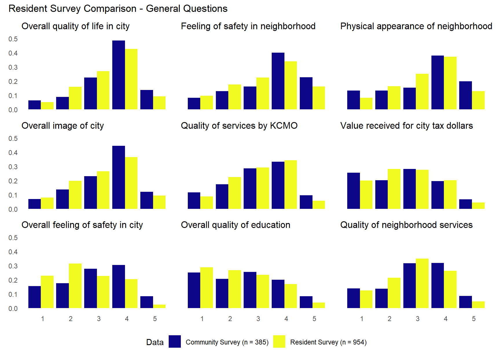
A few things are apparent from the descriptives for the community survey above. First, residents’ perception of the community are generally positive, with averages above the neutral option (3) and medians of 4 for their perceptions of the overall quality of life in the city, safety of their neighborhood, physical appearance of their neighborhood, and overall image of the city. Residents’ perception of the quality of services provided by KCMO, value received for city tax dollars and fees, and overall feelings of safety were somewhat lower, with averages about at the neutral option or lower and medians of 3 (neutral). The lowest average was for residents perceived “value received for city tax dollars and fees.” It was similar for the two questions regarding their overall feelings of safety in their city and their rating of the “quality of police services” with averages and median values around the neutral option. In terms of the questions specifically about “police services,” these too were generally “neutral” in terms of average and median values. The lowest average was for the question asking residents satisfaction with “the city’s overall efforts to prevent crime” while the highest average value was for residents satisfaction with “parking enforcement services.”
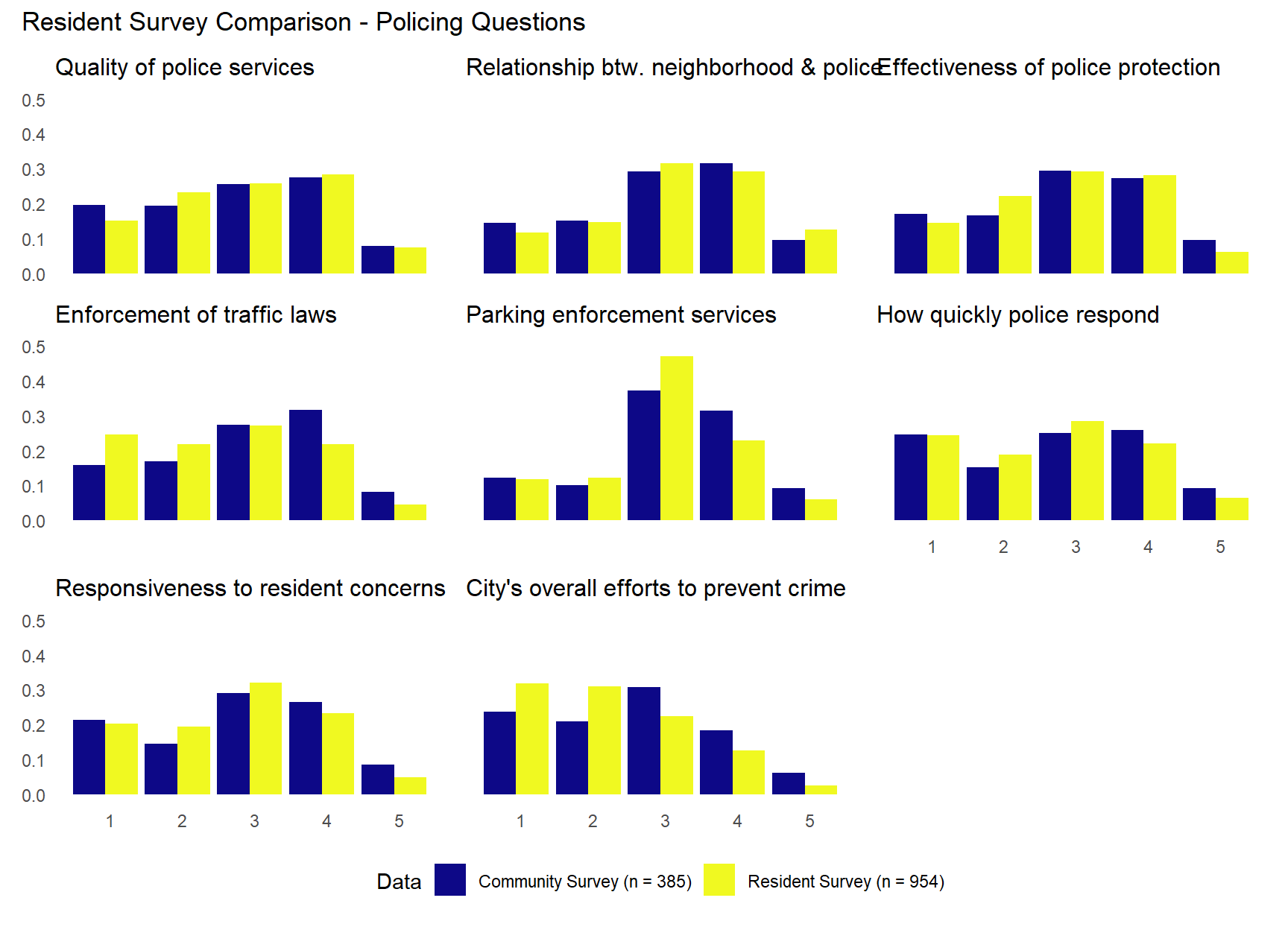
The descriptive results for the fourth quarter resident survey from 2023-2024 are very similar to the community survey. Respondents generally had positive perceptions of the community with average scores above the neutral option for their perceptions of the overall quality of life in the city, safety of their neighborhood, physical appearance of their neighborhood, overall image of the city, and quality of services provided by KCMO. Respondents also generally averaged lower values on value received for city tax dollars and fees, overall feelings of safety, and quality of education. Respondents to the community survey were, on average, more positive about the city than respondents in the resident survey. Results were also similar for the two questions regarding perceptions of the overall quality of neighborhood services and police services with averages at the “neutral” answer category (3). In terms of the questions specifically about “police services,” these too were similar to the community survey but with slightly lower averages. The biggest differences are found between the respondents satisfaction with police “enforcement of local traffic laws” and “the city’s overall efforts to prevent crime.”
Below we will compare the distributions directly, but before doing so, it’s important to recognize the higher missing data rates for the community survey, particularly for some police services questions (e.g., “Parking enforcement services”, “How quickly police respond”, and “Responsiveness to resident concerns”). The relatively large amounts of missing data may influence some of the distributional differences described below.
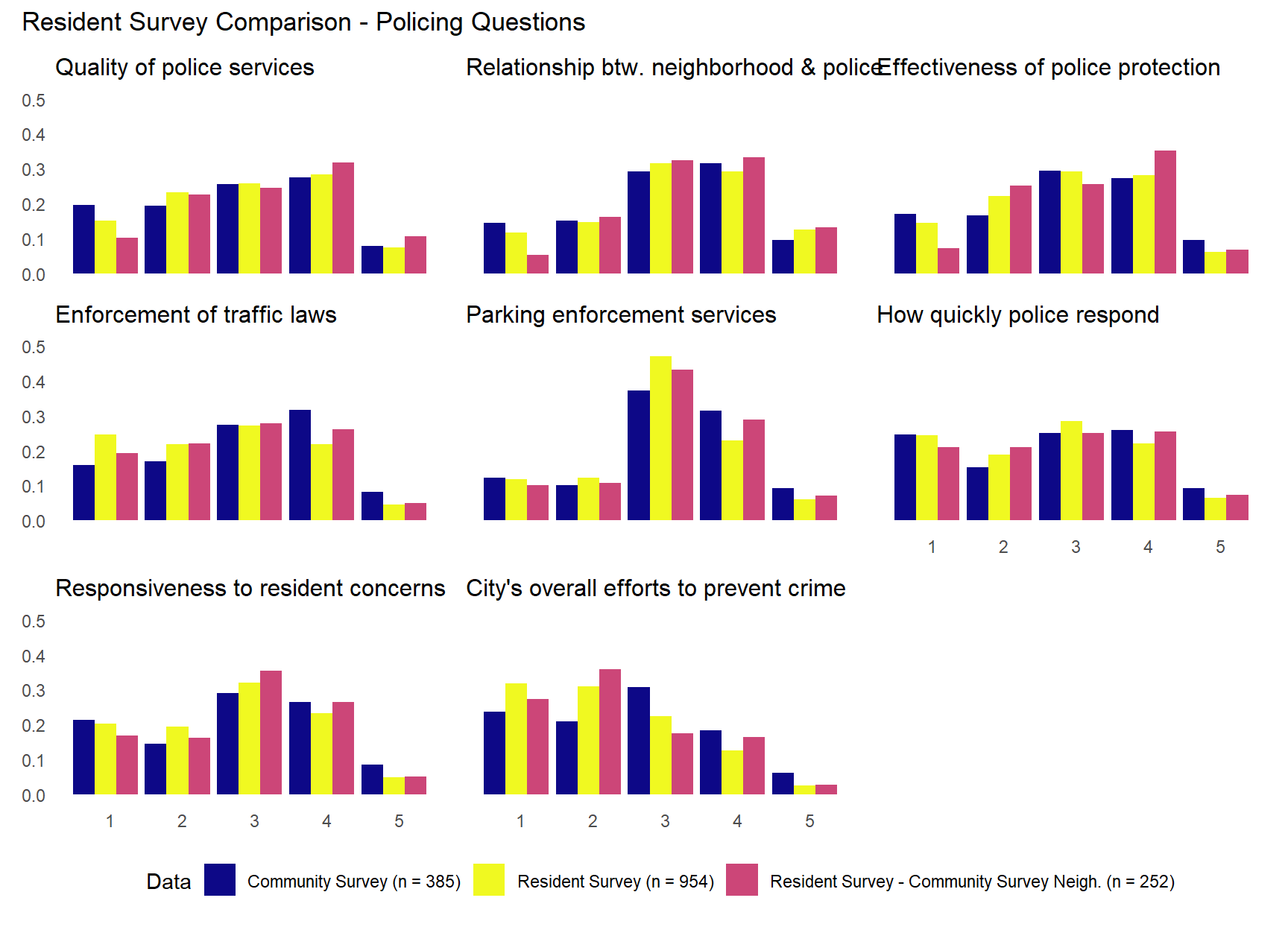
7.0.4 KC Resident Survey Plots
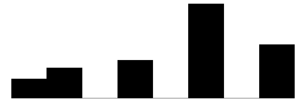
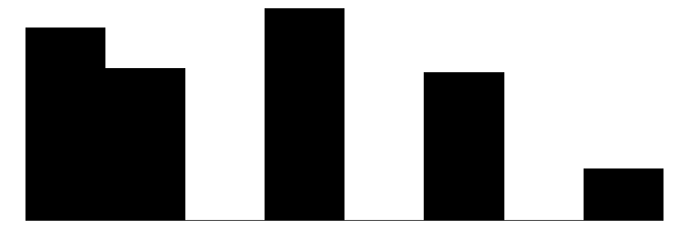
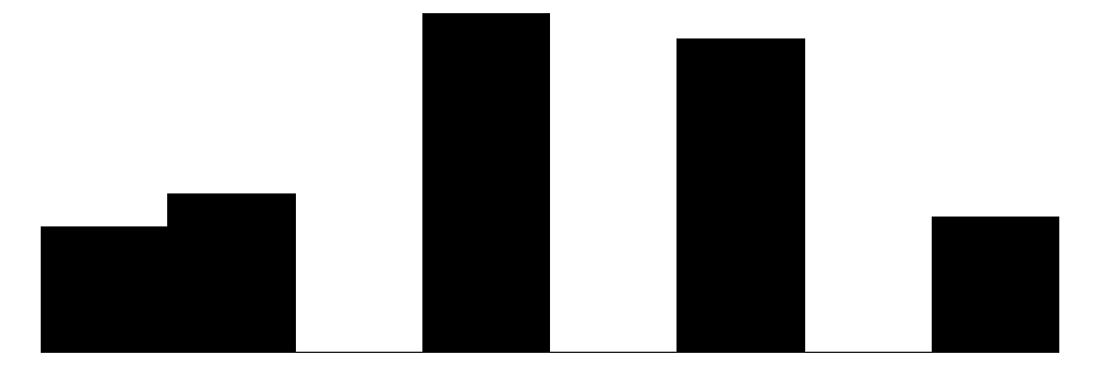
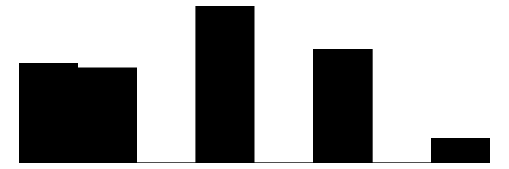
You can get a sense of the similarities and differences across the community and resident survey by looking at the descriptive statistics above, but visualizing their distributions has the potential to be more informative. To do this we will need to produce 17 bar charts with the values of each answer category across the two surveys plotted side-by-side. To make this process as streamlined as possible, we first combine the two data sets with an indicator variable for the survey each observation is associated with.
The plots above suggests that community survey respondents often reported higher satisfaction with quality of life and city image than resident survey respondents. The results were more similar between surveys across the questions dealing with policing. For example, “Quality of police services”, “Relationship between neighborhood & police”, “Effectiveness of police protection”, and “How quickly police respond” questions show remarkably similar distributions across the two surveys. There do appear to be some difference in attitudes toward traffic enforcement. The “Enforcement of traffic laws” question shows community survey respondents slightly more satisfied than resident survey respondents (more category 4 responses) and the “Parking enforcement services” question shows resident survey with notably more category 3 responses, while community survey respondents answer in category 4 and 5 more. The “City’s overall efforts to prevent crime” question shows both samples concentrated in middle categories, but with community survey showing slightly more category 3 responses and resident survey more category 1 and 2 responses. This pattern reinforces the broader finding in the charts above. While both samples show moderate satisfaction overall, the resident survey respondents are somewhat more critical of the city’s crime prevention efforts, rating them in the lower categories more frequently than community survey respondents.
7.0.5 Sampling Disparities: KC Resident vs Community Surveys
The resident survey data includes two geography variables – block_lon and block_lat. These presumably refer to the longitude and latitude of the general location from where each observation resides. We should be able to connect these individual locations to the neighborhood using the “sf” package. This will first require some additional data wrangling with the resident survey data (e.g., scaling the longitude and latitude variables to align with specific geographic coordinate system).
One of the first things we want to examine in the resident survey is how many respondents resided in the 40 neighborhoods included in the community survey. Also of particular interest is how many respondents from the 10 “high crime” neighborhoods responded. One of the goals of the community survey and its design (e.g., using community members as interviewers) was to increase participation from individuals that may be less likely to respond to more traditional surveys like the KC Resident Survey.
As evident in the simple tables above, 17 total responses for the resident survey came from the “high crime” neighborhoods whereas about a quarter of the respondents are located in the randomly sampled neighborhoods from the community survey. Compare this to the Community survey where 88 total respondents (~ 23% of respondents) were from the “high crime” neighborhoods.1
What can these numbers tell us about our community engaged research design? Let’s dig in a little further.
7.0.5.1 Sampling Disparities in Traditional Survey Methods
Of the n=900 total participants in this KC Resident’s Survey quarterly sample, 260 were residents of the 40 neighborhoods in the community survey study. Recall, we classified 10 of these 40 neighborhoods as “high-crime” based on violent crime rates for purposes of stratified random sampling, while 30 were classified as “non-high-crime” sampling strata.
Given this, the sampling patterns show a stark disparity in representation in the KC Resident Survey’s geographic distribution across neighborhood types.
KC Resident Survey sampling rates by neighborhood type:
High-crime neighborhoods: 17 residents across 10 neighborhoods = 1.7 residents per neighborhood (0.65% of total sample per neighborhood)
Non-high-crime neighborhoods: 243 residents across 30 neighborhoods = 8.1 residents per neighborhood (3.12% of total sample per neighborhood)
This represents a 4.8-fold sampling disparity (3.12/0.65 = 4.8), with residents from non-high-crime neighborhoods being nearly five times more likely to participate than residents from high-crime neighborhoods. This pattern is consistent with well-documented challenges in survey research, where communities facing socioeconomic disadvantages, safety concerns, or institutional distrust typically experience lower response rates.
Community Survey sampling rates by neighborhood type:
High-crime neighborhoods: 88 residents across 10 neighborhoods = 8.8 residents per neighborhood (2.37% of total sample per neighborhood)
Non-high-crime neighborhoods: 284 residents across 30 neighborhoods = 9.5 residents per neighborhood (2.55% of total sample per neighborhood)
The community-engaged methodology demonstrates a markedly different sampling pattern that approaches geographic equity. Specifically, the community-engaged approach reduced the sampling disparity to just 1.08-fold, essentially achieving near-parity in representation. This represents a dramatic improvement in sampling equity, transforming a nearly 5-to-1 disparity into virtual equality.
7.0.5.2 Implications for Research Validity and Community Voice
This improvement in geographic representation has important implications for both research validity and democratic participation in municipal research. Traditional survey methods may systematically underrepresent the experiences and perspectives of residents from high-crime neighborhoods, which are precisely the communities most affected by public safety policies and urban challenges.
As desired from the outset, the community-engaged approach’s success in achieving equitable representation suggests that methodological choices significantly impact whose voices are included in research. By training community members as interviewers and building trust through authentic community engagement, the methodology might overcome barriers that limit participation in traditional surveys.
Comparative sampling effectiveness:
Absolute improvement: 88 vs 17 residents from high-crime neighborhoods (5.2x more participants)
Relative probability improvement: 3.5x higher likelihood of participation for high-crime neighborhood residents (.0237/.0065 = 3.6)
Equity improvement: 4.8-fold disparity reduced to 1.08-fold disparity
7.0.5.3 Quantifying sampling disparities: Dissimilarity index
The above figures are probably sufficient for most readers. Yet, bear with us as we get a bit more technical. Social scientists often rely on particular metrics for quantifying varying degrees of inequality (e.g., Gini coefficients; coefficient of variation). One of those is the “dissimilarity index,” which is commonly used to measure segregation and unequal distribution, and it has a pretty intuitive interpretation.
Dissimilarity Index Calculation: Formula: D = (1/2) × Σ|Pi - Qi|
Where:
Pi = proportion of total sample from group i
Qi = proportion that group i “should” have under equal distribution
KC Resident Survey:
High-crime neighborhoods: Should be 10/40 = 25% of community survey subsample, actually 6.5% (17 / 260 = 0.065)
Non-high-crime: Should be 30/40 = 75% of sample, actually 93.5%
The index means 18.5% of the Resident sample and 1.3% of the Community sample would need to be redistributed to achieve perfect geographic proportionality
Dissimilarity reduced from 18.5 to 1.3 using community-engaged methods
93% reduction in geographic inequality (1 - 1.3/18.5 = 0.93)
Conclusion:
This near-elimination of geographic sampling bias provides a more representative foundation for understanding neighborhood social processes and ensures that policy-relevant research reflects the experiences of all community members, not just those most easily reached through conventional methods.
7.0.6 Comparing Survey Results from Same Neighborhoods
Another thing we can do is use this information to provide a more direct comparison of the results from the community survey to the resident survey. Specifically, we can compare the community survey distribution on resident survey variables to the resident survey respondents who resided in the neighborhoods sampled in the community survey.
Resident Survey - Community Survey Neigh. (n = 252)
6
1
3.4
1.0
1.0
4.0
5.0
Feeling of safety in neighborhood
Community Survey (n = 385)
6
5
3.6
1.2
1.0
4.0
5.0
Resident Survey (n = 954)
6
1
3.3
1.2
1.0
4.0
5.0
Resident Survey - Community Survey Neigh. (n = 252)
6
0
3.4
1.2
1.0
4.0
5.0
Physical appearance of neighborhood
Community Survey (n = 385)
6
5
3.4
1.3
1.0
4.0
5.0
Resident Survey (n = 954)
6
1
3.3
1.1
1.0
4.0
5.0
Resident Survey - Community Survey Neigh. (n = 252)
6
1
3.5
1.1
1.0
4.0
5.0
Overall image of city
Community Survey (n = 385)
6
5
3.4
1.1
1.0
4.0
5.0
Resident Survey (n = 954)
6
2
3.2
1.1
1.0
3.0
5.0
Resident Survey - Community Survey Neigh. (n = 252)
6
1
3.2
1.1
1.0
3.0
5.0
Quality of services by KCMO
Community Survey (n = 385)
6
5
3.1
1.2
1.0
3.0
5.0
Resident Survey (n = 954)
6
1
3.1
1.1
1.0
3.0
5.0
Resident Survey - Community Survey Neigh. (n = 252)
6
1
3.1
1.1
1.0
3.0
5.0
Value received for city tax dollars
Community Survey (n = 385)
6
8
2.6
1.2
1.0
3.0
5.0
Resident Survey (n = 954)
6
2
2.6
1.1
1.0
3.0
5.0
Resident Survey - Community Survey Neigh. (n = 252)
6
2
2.6
1.1
1.0
3.0
5.0
Overall feeling of safety in city
Community Survey (n = 385)
6
5
3.0
1.2
1.0
3.0
5.0
Resident Survey (n = 954)
6
1
2.5
1.1
1.0
2.0
5.0
Resident Survey - Community Survey Neigh. (n = 252)
6
1
2.5
1.1
1.0
2.0
5.0
Overall quality of education
Community Survey (n = 385)
6
14
2.7
1.3
1.0
3.0
5.0
Resident Survey (n = 954)
6
17
2.4
1.2
1.0
2.0
5.0
Resident Survey - Community Survey Neigh. (n = 252)
6
16
2.6
1.2
1.0
3.0
5.0
Quality of neighborhood services
Community Survey (n = 385)
6
11
3.1
1.2
1.0
3.0
5.0
Resident Survey (n = 954)
6
9
2.9
1.1
1.0
3.0
5.0
Resident Survey - Community Survey Neigh. (n = 252)
6
7
2.9
1.1
1.0
3.0
5.0
Quality of police services
Community Survey (n = 385)
6
8
2.8
1.2
1.0
3.0
5.0
Resident Survey (n = 954)
6
5
2.9
1.2
1.0
3.0
5.0
Resident Survey - Community Survey Neigh. (n = 252)
6
3
3.1
1.2
1.0
3.0
5.0
Relationship btw. neighborhood & police
Community Survey (n = 385)
6
11
3.1
1.2
1.0
3.0
5.0
Resident Survey (n = 954)
6
12
3.2
1.2
1.0
3.0
5.0
Resident Survey - Community Survey Neigh. (n = 252)
6
12
3.3
1.1
1.0
3.0
5.0
Effectiveness of police protection
Community Survey (n = 385)
6
8
3.0
1.2
1.0
3.0
5.0
Resident Survey (n = 954)
6
8
2.9
1.1
1.0
3.0
5.0
Resident Survey - Community Survey Neigh. (n = 252)
6
8
3.1
1.1
1.0
3.0
5.0
Enforcement of traffic laws
Community Survey (n = 385)
6
8
3.0
1.2
1.0
3.0
5.0
Resident Survey (n = 954)
6
7
2.6
1.2
1.0
3.0
5.0
Resident Survey - Community Survey Neigh. (n = 252)
6
6
2.8
1.2
1.0
3.0
5.0
Parking enforcement services
Community Survey (n = 385)
6
12
3.2
1.1
1.0
3.0
5.0
Resident Survey (n = 954)
6
21
3.0
1.0
1.0
3.0
5.0
Resident Survey - Community Survey Neigh. (n = 252)
6
24
3.1
1.0
1.0
3.0
5.0
How quickly police respond
Community Survey (n = 385)
6
13
2.8
1.3
1.0
3.0
5.0
Resident Survey (n = 954)
6
21
2.7
1.2
1.0
3.0
5.0
Resident Survey - Community Survey Neigh. (n = 252)
6
22
2.8
1.2
1.0
3.0
5.0
Responsiveness to resident concerns
Community Survey (n = 385)
6
12
2.9
1.3
1.0
3.0
5.0
Resident Survey (n = 954)
6
18
2.7
1.2
1.0
3.0
5.0
Resident Survey - Community Survey Neigh. (n = 252)
6
17
2.9
1.1
1.0
3.0
5.0
City's overall efforts to prevent crime
Community Survey (n = 385)
6
8
2.6
1.2
1.0
3.0
5.0
Resident Survey (n = 954)
6
5
2.2
1.1
1.0
2.0
5.0
Resident Survey - Community Survey Neigh. (n = 252)
6
6
2.3
1.1
1.0
2.0
5.0
data_fact
N
%
Community Survey (n = 385)
385
24.1
Resident Survey (n = 954)
954
59.7
Resident Survey - Community Survey Neigh. (n = 252)
260
16.3
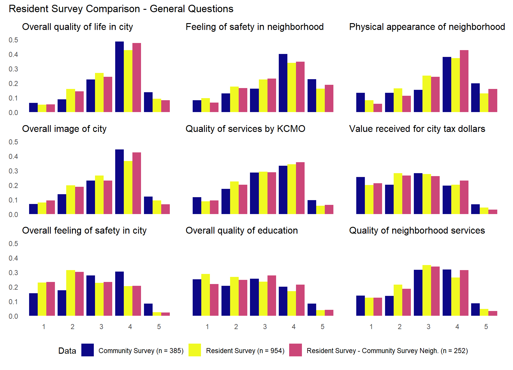
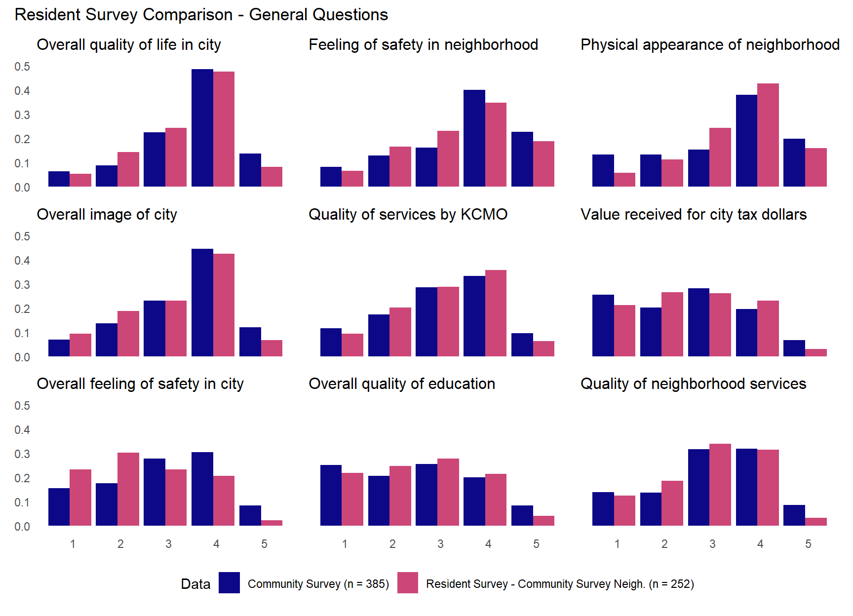
The table above shows the descriptives by each sample (or subsample). The three (sub)samples show very similar community sentiment. Most variables show means within 0.1-0.3 points of each other. Where there are (small) differences, the community survey tends to show higher (more positive) mean values.
We can also plot these differences similar to what we did with the full resident survey sample above.
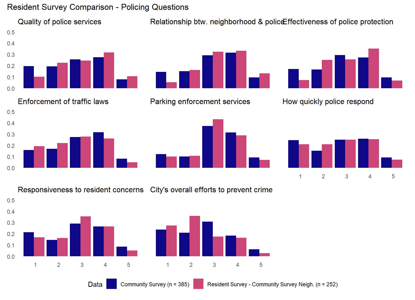
The plots above show the distributions of all three (sub)samples. They largely confirm the similarity across the different (sub)samples. Although there is some evidence that the community survey sample and sub-sample from the same neighborhoods in the residents survey are more similar to each other than the overall resident survey sample. They also tend to be somewhat more positive about the overall “quality of life” and “image of” the city as well as “feelings of safety” in and perceived “physical appearance” of their neighborhoods (Note the similar and larger peaks in values of 4 compared to the full resident survey). For the policing-related questions, there is some evidence that the resident survey sub-sample of community survey neighborhoods shows more positive perception of the overall “quality of police services,” “relationship between neighborhood and police,” and “quality of police protection.” Community-survey respondents tend to have slightly higher but perhaps more variation in their perception of traffic and parking enforcement services while the sub-sample of community survey neighborhoods from the resident survey is more concentrated in the middle value. For the questions regarding police response times and their responsiveness to resident concerns, the community survey shows a slightly more negative skew than the sub-sample from the resident survey where the opposite is true for the question regarding the city’s overall effort at crime prevention.
By plotting results for three different (sub)samples on the same plots, the figures above can be a little difficult to interpret. Given our main focus is to compare the results of the community survey to the results from the resident survey administered in the same neighborhoods, let’s just plot that comparison.
7.0.7 Comparing response-level estimation across samples
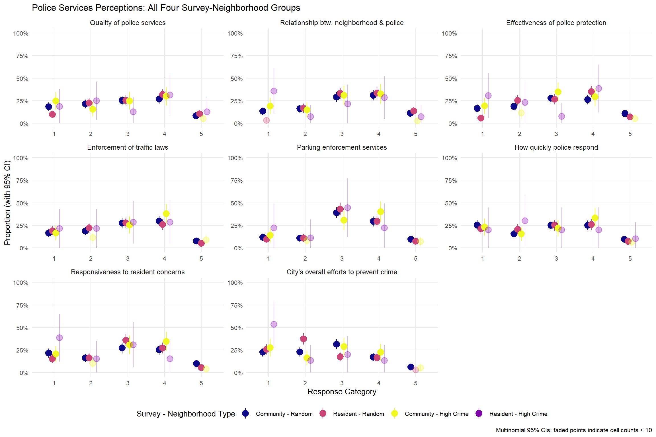
Now, bear with us as we dig a little deeper. Specifically, we will compare our ability to precisely estimate basic univariate statistics - like the response proportions shown in the bar charts above - across the KC Community and Resident “random” and “high crime” samples. To do this, we will compare estimates and 95% confidence intervals derived from the Community survey and the quarterly Resident survey data separately for the 30 “random sample” neighborhoods and the 10 “high crime” neighborhoods using the same items we described above. This is important because it will allow us to further assess whether the community-engaged approach improved our ability to study residents in those high crime neighborhoods that were under-represented in the resident data generated using more traditional survey methods.
Show code
# Check cell counts by response category for each group# cell_counts_check <- kc_comres_stratified %>%# select(all_of(general_vars), survey_strata_fact) %>%# pivot_longer(cols = all_of(general_vars), names_to = "variable", values_to = "value") %>%# filter(!is.na(value)) %>%# group_by(variable, survey_strata_fact, value) %>%# summarise(cell_count = n(), .groups = "drop") %>%# group_by(variable, survey_strata_fact) %>%# mutate(# total_n = sum(cell_count),# proportion = cell_count / total_n# ) %>%# ungroup()# Look at a specific variable to see the pattern# cell_counts_check %>%# filter(variable == "percom_quallife") %>%# arrange(survey_strata_fact, value) %>%# print(n = 50)# Summary of cell counts across all variables# cell_counts_check %>%# group_by(survey_strata_fact) %>%# summarise(# min_cell_count = min(cell_count),# max_cell_count = max(cell_count),# median_cell_count = median(cell_count),# mean_cell_count = mean(cell_count),# .groups = "drop"# )
    Community Survey - Random Sample      Resident Survey - Random Sample
                                 284                                  243
Community Survey - High Crime Sample  Resident Survey - High Crime Sample
                                  88                                   17
                                <NA>
                                   0
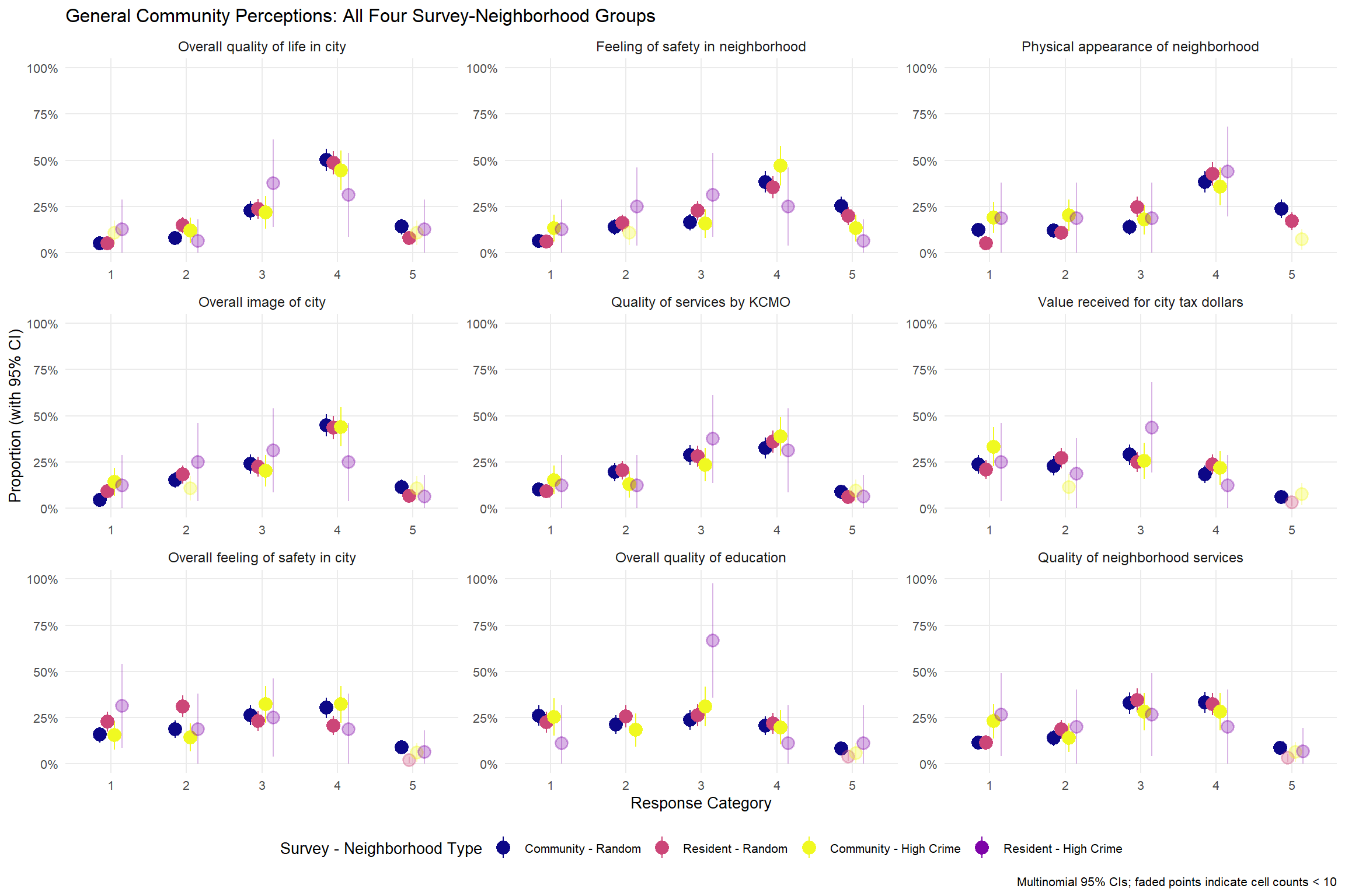
Above, we conducted a comparative analysis examining response patterns across four distinct survey-neighborhood groups: Community Survey from random sample neighborhoods (n=285), Resident Survey from random sample neighborhoods (n=243), Community Survey from high-crime neighborhoods (n=88), and Resident Survey from high-crime neighborhoods (n=17).2 Rather than simply comparing means, we calculated the proportion of responses in each category (1-5 on the satisfaction scale) for each group and estimated 95% confidence intervals around these proportions using multinomial standard errors.
The resulting plots display these proportions with confidence intervals as point-range estimates, positioned along the x-axis by response category and faceted by survey question. Points are color-coded by survey-neighborhood combination and faded when cell counts fall below 10 observations to indicate high uncertainty. This approach reveals not just differences in response patterns between groups, but also the reliability of those differences–showing, for example, that the Resident Survey high-crime group (with only 17 total respondents) produces much wider confidence intervals than the larger Community Survey groups, particularly for rare response categories. Overall, the visualizations provide both substantive insights about how survey methodology and neighborhood type affect resident perceptions, and methodological insights about where sample sizes are sufficient to support confident conclusions versus where uncertainty remains high.
First, perhaps the most immediately apparent (and anticipated) pattern is that the Resident survey - High Crime sample (n=15-17 across questions) shows dramatically wider confidence intervals than all other groups, with many intervals spanning 30-40 percentage points. Nearly every estimate for this group is flagged as a small cell (count < 10), highlighting the fundamental uncertainty in these estimates. In comparison, the Community survey - High Crime sample typically generated much more precise estimates (i.e., narrower confidence intervals), even for low-prevalence response categories with small cell counts.
Second, this disaggregated analysis reveals patterns that are remarkably consistent across the other three survey sample/method conditions. When focusing specifically on the two comparable random sample groups (Community vs. Resident), the patterns are remarkably similar across most questions, with largely overlapping confidence intervals. For example, on “Overall quality of life in city,” both groups show their highest proportions in category 4 (Community: 50%, CI: 44-56%; Resident: 49%, CI: 42-55%), suggesting that the community-engaged survey approach produces minimal bias relative to the traditional Resident survey when neighborhood context is held constant. Similar convergence appears for “Physical appearance of neighborhood” and most policing-related questions, validating the community survey methodology.
With that said, though survey method effects appear minimal when neighborhood type is held constant, the Community Survey’s adequate sample sizes reveal potentially important differences between high-crime and random sample neighborhoods that the traditional resident survey could not reliably detect:
Neighborhood Safety Perceptions: “Feeling of safety in neighborhood” also reveals differences when examining individual response categories. Community Survey respondents in High-crime neighborhoods are more than twice as likely to report being very dissatisfied (category 1: 13%, CI: 6-21%) compared to random sample respondents (6%, CI: 3-9%). At the other extreme, residents of high-crime neighborhoods are much less likely to report being very satisfied (category 5: 13%, CI: 6-21%) compared to residents of randomly sampled neighborhoods (26%, CI: 20-31%)–essentially a complete reversal of proportions between the most and least satisfied categories. The modal response also differs meaningfully: random sample neighborhood residents most commonly choose category 4 (38%, CI: 32-44%), while high-crime neighborhood residents’ responses show a flatter distribution with category 4 still highest (47%, CI: 36-58%) but much higher proportions in categories 1-3 combined (53% vs. 36% in random sample).
Appearance of Physical Environment: Community Survey residents in high-crime neighborhoods report nearly twice the rate of strong dissatisfaction with neighborhood appearance (category 1: 19%, CI: 11-27%) compared to random sample residents (12%, CI: 8-16%), while showing much lower rates of high satisfaction (category 5: 7%, CI: 2-13%) versus random sample (24%, CI: 19-29%).
Municipal Service Satisfaction: Two municipal service questions reveal perceived neighborhood-level disparities. On “Value received for city tax dollars,” 33% (CI: 23-44%) of Community Survey residents in high-crime neighborhoods reported the most dissatisfied category versus 24% (CI: 18-29%) in random neighborhoods–a difference with relatively low confidence interval overlap. Similarly, “Quality of neighborhood services” shows high-crime respondents reporting 23% in the most dissatisfied category (CI: 14-32%) compared to 11% in random neighborhoods (CI: 8-15%).
Policing: Most policing questions show minimal differences across neighborhood types. For example, looking at “Relationship btw. neighborhood & police,” the patterns are actually quite similar between high-crime and random neighborhoods in the Community Survey. High-crime respondents show 32% in category 4 (CI: 22-43%) compared to 31% in random sample (CI: 25-36%). The satisfaction levels (categories 4-5 combined) are 35% for high-crime vs. 42% for random sample - a modest difference but with overlapping confidence intervals. Similarly, across “Effectiveness of police protection,” “How quickly police respond,” “Enforcement of traffic laws,” and “Parking enforcement services,” the differences between high-crime and random neighborhoods are generally small and confidence intervals overlap substantially. The “Quality of police services” item similarly shows comparable patterns - high-crime respondents have 30% in category 4 (CI: 20-40%) vs. 27% in random sample (CI: 21-32%), with high-crime residents actually reporting slightly higher satisfaction in the top category. One possible exception is with crime prevention, where the “City’s overall efforts to prevent crime” item shows residents of high-crime neighborhoods are more likely to be in the most dissatisfied category (28% vs. 22% in random sample), though confidence intervals still substantially overlap (CI: 18-37% vs. 17-27%).
These patterns suggest that Community Survey methodology not only provides more reliable estimates for high-crime neighborhoods but also reveals substantively important differences in resident experiences that traditional surveys cannot detect due to inadequate sample sizes. Interestingly, police-related satisfaction showed minimal differences between neighborhood types, contrasting sharply with differences observed in safety perceptions, physical appearance, and municipal services. Importantly, many apparent differences between survey methods in high-crime neighborhoods cannot be reliably assessed due to the inadequate Resident Survey sample size, underscoring how traditional survey approaches might systematically under-represent precisely those communities most affected by municipal policies.
7.0.8 Conclusion
This comparative analysis of the KC Community Survey and Resident Survey reveals both consistencies and meaningful differences in how Kansas City residents perceive their community and city services. The comparison demonstrates that the community survey methodology successfully captured resident sentiment that closely aligns with the established resident survey, while also providing valuable insights into previously underrepresented neighborhoods. Most importantly, the analysis appears to reveal fundamental limitations in the KC Resident Survey’s traditional survey methods’ ability to reliably capture perspectives from high-crime neighborhoods due to inadequate sample sizes–a limitation largely overcome by the KC Community Survey’s community-engaged methodology.
7.0.8.1 Key Findings
The most significant finding is the remarkable similarity in response patterns between the two surveys, particularly on policing-related questions. Items measuring “Quality of police services,” “Relationship between neighborhood & police,” “Effectiveness of police protection,” and “How quickly police respond” showed very similar distributions across both surveys. This consistency validates the community survey’s ability to similarly capture resident perspectives on police services, which was a primary objective given the focus on high-crime neighborhoods. Notably, when examining neighborhood differences within the Community Survey, police-related satisfaction showed minimal variation between high-crime and random sample neighborhoods, contrasting with other domains where some neighborhood differences were observed.
However, notable differences emerged in residents’ perceptions of general community attributes. Community survey respondents consistently reported higher satisfaction with quality of life indicators, including overall quality of life in the city, the city’s image, and feelings of safety in their neighborhoods. These differences were most pronounced when comparing the community survey to the full resident survey sample, but persisted even when limiting the comparison to resident survey respondents from the same neighborhoods. The Community Survey’s adequate sample sizes revealed potentially meaningful neighborhood differences in areas such as safety perceptions, neighborhood physical appearance, and municipal services–differences that traditional surveys cannot reliably detect due to insufficient representation from high-crime neighborhoods.
Importantly, uncertainty analysis using confidence intervals around response proportions reveals that many apparent differences between survey methods in high-crime neighborhoods cannot be reliably assessed due to the Resident Survey’s inadequate sample sizes (n=15-17), which produced confidence intervals spanning 30-40 percentage points compared to the much more precise estimates from the Community Survey’s larger high-crime sample (n=88).
7.0.8.2 Geographic and Methodological Implications
The geographic analysis reveals an important achievement of the community survey design. While only 17 respondents from high-crime neighborhoods participated in the resident survey (representing a small fraction of the total sample), the community survey successfully engaged 88 respondents from these same neighborhoods—comprising nearly a quarter of all community survey responses. This demonstrates that the community-based interviewing approach effectively reached residents who may be less likely to participate in traditional mail, phone, and online surveys.
The similarity between the community survey results and the resident survey sub-sample from the same neighborhoods (n=252) further supports the community survey methodology. When controlling for geographic location, the two surveys produced remarkably consistent results, with most mean differences falling within 0.1-0.3 points on the 5-point scale and with uncertainty analysis showing remarkably similar response patterns. This consistency is particularly notable given that both random sample groups achieved sufficient sample sizes to produce reliable estimates with overlapping confidence intervals.
7.0.8.3 Limitations and Considerations
Several limitations should be acknowledged. The resident survey data represents only the fourth quarter of fiscal year 2023-2024 rather than the full annual sample, which may limit generalizability. Additionally, the community survey showed higher rates of missing data on certain police services questions, particularly for parking enforcement and police response times, which may reflect different levels of direct experience with these services across neighborhoods.
The slightly more positive responses in the community survey could reflect multiple factors: the face-to-face interview format may elicit more socially desirable responses, the community-based interviewers may have established better rapport with respondents, or residents in the sampled neighborhoods may genuinely have more positive perceptions than initially expected. However, uncertainty analysis suggests these differences are often within the range of statistical noise when sample sizes are small.
7.0.8.4 Implications for Future Research and Policy
These findings suggest that the community survey successfully accomplished its primary objectives: engaging residents from high-crime neighborhoods who are typically underrepresented in traditional surveys while maintaining methodological rigor that produces reliable, comparable data. The uncertainty analysis demonstrates that this is not merely a matter of inclusion, but of statistical necessity, as traditional surveys may be unable to provide policy-relevant insights about high-crime neighborhoods due to fundamental sample size limitations without explicit modification (e.g., purposive oversampling).
For future iterations, researchers should prioritize ensuring adequate sample sizes across all neighborhood types rather than relying on population-proportionate sampling that systematically underrepresents policy-critical communities. The methodology appears particularly well-suited for gathering authentic community input on sensitive topics like policing, where both representation and statistical precision are essential for evidence-based policymaking.
7.0.8.5 Final Thoughts
This analysis demonstrates that thoughtful survey design can successfully bridge the gap between rigorous social science methodology and authentic community engagement. The community survey not only validated existing resident survey findings but also provided crucial insights from neighborhoods that are often underrepresented in municipal decision-making processes. As Kansas City continues to address issues of public safety, community development, and municipal service delivery, this enhanced understanding of resident perspectives across all neighborhoods provides a more complete foundation for evidence-based policymaking.
Kuriakose, Noble, and Michael Robbins. 2015. “Don’t GetDuped: Fraud Through Duplication in PublicOpinionSurveys.” {SSRN} {Scholarly} {Paper}. Rochester, NY: Social Science Research Network. https://papers.ssrn.com/abstract=2580502.
Revelle, William. 2024. “The Seductive Beauty of Latent Variable Models: Or Why I Don’t Believe in the EasterBunny.”Personality and Individual Differences 221 (April): 112552. https://doi.org/10.1016/j.paid.2024.112552.
Sampson, Robert J., Stephen W. Raudenbush, and Felton Earls. 1997. “Neighborhoods and ViolentCrime: AMultilevelStudy of CollectiveEfficacy.”Science 277 (5328): 918–24. https://doi.org/10.1126/science.277.5328.918.
Note: in the table above, 13 respondents are excluded from the community survey frequencies. These 13 respondents are from the online version of the community survey who were coded with NBHD = 43, which did not have a corresponding official neighborhood.↩︎
Note that analytical sample sizes vary depending on missing data patterns.↩︎