13  Appendix IV - Power Analysis

13.1 Introduction

This appendix includes the a priori power analysis provided for Maja to help her consider implications of her initial research design. In brief, she was securing resources to interview approximately n=800 residents of 40 KC neighborhoods, with a target sample size of approximately 20 participants per neighborhood. She wanted to know if that design would provide sufficient statistical power to examine various individual- and neighborhood-level differences (e.g., in collective efficacy; perceptions of police; general perceptions). Given initial preferences regarding the target sample size and lacking a specific target test hypothesis for which I could specify a reasonably precise modeling approach and plausible range of effect sizes, I took a different approach. Specifically, in this power analysis, I attempted to answer the following question:

“Given the research design, Likert-type ordinal data likely to be collected, and research focus on ‘high-crime’ and”non-high-crime” neighborhoods, what are some typical effect sizes (e.g., contrasts in ‘agreement’ rates between high-crime and random sample neighborhoods in terms of odds ratios and predicted probabilities or percentage-point differences) that I might expect a priori to be able to detect with adequate (≥80%) power?”

In brief, the analysis concluded:

“Based on these simulations, the proposed design (n=800, 40 neighborhoods, 20 participants per neighborhood) provides adequate power (≥80%) to detect effect sizes of OR=1.35 or larger. In practical terms, this corresponds to detecting differences of approximately 6-9 percentage points in ‘agreement’ rates between high-crime and random sample neighborhoods.”

13.2 Assumptions

Assume we can meaningfully distinguish at the outset between adults in high risk neighborhoods from those in non-high risk neighborhoods; high risk neighborhoods experience high rates of serious violent and property crimes and, as such, are likely targets for anti-crime interventions. Assume, too, that we want to know if there are substantively meaningful differences across these neighborhood risk levels in various things such as adult residents’ involvement in neighborhood organizations, their perceived agreement with the neighborhood or with police services, or reported indicators of collective efficacy (e.g., social control; cohesion) in the neighborhood.

Let’s use a couple concrete examples from the PHDCN’s community survey for our power analysis.

People might differ in the degree to which residents perceive that people in their neighborhood can be trusted or that people are willing to help their neighbors, and residents of “not at risk” (i.e., lower crime) neighborhoods might report greater agreement with such statements than those in “at risk (i.e., higher crime) neighborhoods.

The PHDCN community survey contains a series of questions like this to measure dimensions of collective efficacy using ordinal responses ranging from strongly agree (=1) to strongly disagree (=5). Here are aggregated distributions for valid responses on these two particular items:

Q11E. people are willing to help their neighbors

• agree (=1,2): 74.4%
• do not agree (=3,4,5): 25.6%

Q11M. people can be trusted

• agree (=1,2): 60.1%
• do not agree (=3,4,5): 39.9%

The KC community survey will contain many comparable items and, ultimately, we plan to use ordinal modeling techniques to assess differences in individual item response distributions like these across neighborhoods. Despite planning to build ordinal models, we anticipate our final public report will probably collapse and present dichotomous differences in the probability of reporting “agreement” (like the PHDCN aggregated example above) across at-risk and not-at-risk neighborhoods for accessible presentation to non-academic audiences. So, we want to take this into consideration when conducting a power analysis.¹

Let’s also assume that, with oversampling high risk neighborhoods, 50% of our sample is high risk (p1=0.50). This might be a high estimate (e.g., 50% of neighborhoods might not plausibly be considered for anti-crime interventions). However, examination of 2023 KC neighborhood crime rate data shows about 60% (149/237) of neighborhoods have single-digit violence crime rates per 1000 and about 40% (88/237) have double-digit violence rates. By design, 10 of the “at-risk” neighborhoods with the highest violence rates are included via oversampling. Then, stratified probability sampling procedures for identifying the other 30 neighborhoods is expected to yield another 10 “at risk” neighborhoods (78/227 = 0.34; 0.34*30 = 10.2), which would result in approximately an even split between “at risk” (double-digit violence rates) and “not at risk” neighborhoods in the KC sample. Note that, given funding and levels of concern, perhaps a smaller group is really under consideration for intervention at any given time; however, by overestimating and oversampling the “at risk” group (and thus assuming more equivalent group proportions), we anticipate generating more conservative power estimates (i.e., by maximizing variability).

Thus, for this a priori power analysis, we seek to estimate our statistical power to detect differences of varying magnitudes in analyses that are akin to those described above, given a fixed research design with the following parameters:

• alpha level of 0.05
• total n=800 participants
• total of 40 neighborhoods, with 20 participants per neighborhood
• p(“at risk” neighborhood) = p(x=0) = 0.5
• group sizes of n1=400 and n2=400 (0.5*800)

Though seemingly a simple question, this is somewhat complicated to determine given our anticipated models and estimands. As a result, instead of using power calculators, we will estimate power using a simulation approach.

13.3 Simulated data & model testing

With our simulation approach, we want to estimate whether ordinal response distributions (e.g., degree of agreement) differ across “at risk” (x=0) and “not at risk” (x=1) neighborhoods; for this, we will rely on ordinal (e.g., cumulative logit) regression thresholds and beta coefficients. Ultimately, we will collapse these ordinal distributions into dichotomies (e.g., “agree”/“not agree”) for the purposes of reporting basic differences across neighborhoods.

Let’s first try to simulate some plausible data, then build a model and visualize the focal contrast. If we can do this, then we should be able to reiterate the process repeatedly under particular parameter settings to compare power estimates across effect sizes at fixed sample sizes and alpha levels. For this initial simulation, we start by assuming the true difference across groups is represented by an odds ratio of about 1.5, which would equate to a log odds coefficient of log(1.5) = 0.41.

How big is this difference? Well, let’s do some rough calculations to consider what this effect size (OR=1.5) might look like if we, say, subtract 0.03, from the probabilities reflected in those PHDCN items above to use as baseline probabilities (i.e., as the expected probability of agreement when x=0).

Q11E. people are willing to help their neighbors

• overall probability of agreement: 0.75
• assumed baseline probability of agreement (when x=0): 0.72
• baseline odds of agreement in x=0[at risk]: 0.72/0.28 = 2.57
• Odds of agreement in x=1[not at risk]: (2.57)x(1.5) = 3.86
• P(agree|x=0[at risk]) = odds/(1+odds) = 2.57/(1+2.57) = 0.72 (conversion works)
• P(agree|x=1[not at risk]) = odds/(1+odds) = 3.86/(1+3.86) = 0.79
• p(agree|x=1) - p(agree|x=0) = 0.79 - 0.72 = .06 = 6 percentage point difference in “agreement” (i.e., y=1 and y=2) responses across groups

Q11M. people can be trusted

• overall probability of agreement: 0.60
• assumed baseline probability of agreement (when x=0): 0.57
• assumed baseline odds of agreement: 0.57/0.43 = 1.33
• Odds of agreement in x=1[not at risk]: (1.33)x(1.5) = 2.0
• P(agree|x=0[at risk]) = odds/(1+odds) = 1.33/(1+1.33) = 0.57 (conversion works)
• P(agree|x=1[not at risk]) = odds/(1+odds) = 2.0/(1+2.0) = 0.67
• p(agree|x=1) - p(agree|x=0) = 0.67 - 0.57 = .10 = 10 percentage point difference in “agreement” (i.e., y=1 and y=2) responses across groups

So, in this context, an OR=1.5 might be a small to medium difference on a probability scale (e.g., 6 to 10 percentage point absolute difference across groups), depending on the specific ordinal item response distributions.

One final word about assumptions. In our simulation below, we will assume baseline ordinal response distributions vary randomly across individuals and to a lesser extent neighborhoods, and responses are systematically “higher” (more agreeable) in not-at-risk neighborhoods (OR=1.5). Additionally, the PHDCN’s collective efficacy items showed higher “agreement” (strongly agree & agree) than “non-agreement” responses. So, in our simulation, items are reverse-coded such that our higher values equal greater agreement (or satisfaction or involvement), then cumulative logit cutpoints that are assymmetric around the middle category (y=3) are specified such that more probability mass is placed on the higher (agree) categories. Specifically, the cutpoints approximately translate to the following baseline probabilities:

• p(SD or y=1) = 0.182
• p(D or y=2) = 0.195
• p(N or y=3) = 0.123
• p(A or y=4) = 0.318
• p(SA or y=5) = 0.182

These baseline probabilities correspond to the following cumulative logit cutpoints:

cumulative_probs <- c(0.182, 0.377, 0.5, 0.818)

# Calculate cutpoints using the inverse logit function (qlogis)
cutpoints <- qlogis(cumulative_probs)

# Print the cutpoints
cutpoints

[1] -1.5028556 -0.5023013  0.0000000  1.5028556

• cp1 = 0.182; cutpoint = -1.5
• cp2 = 0.377; cutpoint = -0.5
• cp3 = 0.5; cutpoint = 0
• cp4 = 0.818; cutpoint = 1.5

Now, let’s try simulating one dataset to see if we can estimate power given these assumptions.

13.3.1 example sim to test

library(lme4)
library(ordinal)
library(tidyverse)

set.seed(1138)

# Set the parameters
n_neigh <- 40  # Number of neighborhoods
n_ind <- 20    # Number of individuals per neighborhood
n <- n_neigh * n_ind  # Total number of individuals
beta0 <- 0     # Intercept
beta1 <- log(1.5)  # Effect size (log-odds for binary x)
sigma_neigh <- .25  # Neighborhood random effect standard deviation
sigma_ind <- 1  # Individual-level noise

# Simulate binary predictor ensuring equal split
x_neigh <- rep(c(0, 1), each = n_neigh / 2)  # 20 "at risk" and 20 "not at risk"

# Simulate neighborhood IDs
neigh_id <- rep(1:n_neigh, each = n_ind)

# Assign neighborhood-level x to individuals
x <- rep(x_neigh, each = n_ind)

# Generate neighborhood-level random intercepts
neigh_intercept <- rnorm(n_neigh, mean = 0, sd = sigma_neigh)

# Individual-level noise
ind_noise <- rnorm(n, mean = 0, sd = sigma_ind)

# Linear predictor (latent continuous variable)
linpred <- beta0 + beta1 * x + neigh_intercept[neigh_id] + ind_noise

# Cut points (thresholds) for the ordinal outcome (logit-scale)
cutpoints <- c(-1.5, -0.5, 0, 1.5)

# Use the cut() function to assign categories
y <- cut(linpred, breaks = c(-Inf, cutpoints, Inf), labels = 1:5, ordered_result = TRUE)

# Combine into a data frame
simdat <- data.frame(
  neigh_id = neigh_id,
  x = factor(x),  # Binary neighborhood predictor as factor
  y = factor(y, ordered = TRUE)  # Ordinal response variable
)

# Check distribution
print("Distribution of x:")

[1] "Distribution of x:"

print(table(simdat$x))

  0   1 
400 400 

print("Distribution of y:")

[1] "Distribution of y:"

print(table(simdat$y))

  1   2   3   4   5 
 30 164 152 374  80 

We have data! Now, let’s visualize the differences in ordinal distributions across groups using a mosaic plot.

13.3.2 visualize ordinal distribution contrast

library(ggmosaic)
library(viridis)

mosyplot <- function(df, yvar, xvar, xlabel, ylabel, mytitle, mysubtitle){
  ggplot() +
  geom_mosaic(data=df, aes(x = product(!!as.name(yvar), !!as.name(xvar)), fill = !!as.name(yvar)),
              na.rm=TRUE) +
  labs(x = xlabel,
       y = ylabel,
       title=mytitle,
       subtitle = mysubtitle) +
  scale_fill_viridis_d(begin=.1, end=.9, direction=-1,
                       option="magma", 
                       guide = guide_legend(reverse = TRUE)) +
  theme_minimal() +
  theme(panel.grid.major = element_blank(),
        panel.grid.minor = element_blank(),
        axis.text.y = element_blank())
  }

ordplot <- mosyplot(df=simdat, "y", "x", "Neighborhood risk",
         "Proportion satisfied", "Mosaic plot y by x",
         "Left to Right = (0) at risk / (1) not at risk"
)
ordplot

Everything appears to have worked, and it appears from this graph that the “not at risk” (x=1) neighborhood group actually shows greater overall agreement responses (y=4,5) than the “at risk” (x=0) neighborhoods. It is not clear whether these observed differences recovered the specified parameter’s magnitude (OR=1.5). Let’s fit a cumulative logit model with a neighborhood risk predictor and a neighborhood random effect to estimate the effect in this particular sample.

13.3.3 build (frequentist) model

# Fit the cumulative link mixed model (CLMM) with neighborhood random effects
fit <- clmm(y ~ x + (1 | neigh_id), data = simdat)
summary(fit)

Cumulative Link Mixed Model fitted with the Laplace approximation

formula: y ~ x + (1 | neigh_id)
data:    simdat

 link  threshold nobs logLik   AIC     niter    max.grad cond.H 
 logit flexible  800  -1072.19 2156.39 319(648) 2.74e-05 1.9e+02

Random effects:
 Groups   Name        Variance Std.Dev.
 neigh_id (Intercept) 0.0382   0.1954  
Number of groups:  neigh_id 40 

Coefficients:
   Estimate Std. Error z value Pr(>|z|)    
x1   0.4887     0.1458   3.352 0.000804 ***
---
Signif. codes:  0 '***' 0.001 '**' 0.01 '*' 0.05 '.' 0.1 ' ' 1

Threshold coefficients:
    Estimate Std. Error z value
1|2  -3.0470     0.1999 -15.245
2|3  -0.9197     0.1114  -8.255
3|4  -0.0318     0.1058  -0.301
4|5   2.4825     0.1484  16.723

In our (frequentist) cumulative logit model applied to this particular simulated dataset, we estimated a log odds coefficient of 0.489, which equates to an odds ratio of 1.58 (exp[0.457]=1.63). This is close to recovering our simulated parameter of log(1.5).

The coefficient is also statistically significant at alpha=0.05. But, this is one sample, and the estimate is a little larger than the parameter. Is our design able to reliably estimate confidence intervals that will contain an effect of OR=1.5 at an alpha level of 0.05 with 80% power?

13.4 Power analysis

To answer this, we can iterate our simulation 100 times and then count the number that detect a statistically significant effect. If that number is >=80 (out of 100, or 80%), then we can infer via simulation that our statistical power is >= 0.80.

13.4.1 est. power for OR=1.5

# Set simulation parameters
n_sim <- 100  # Number of simulations
alpha <- 0.05  # Significance level for hypothesis test

# Set the parameters for each simulation
n_neigh <- 40  # Number of neighborhoods
n_ind <- 20    # Number of individuals per neighborhood
n <- n_neigh * n_ind  # Total number of individuals
beta0 <- 0     # Intercept
beta1 <- log(1.5)  # Effect size (log-odds for binary x)
sigma_neigh <- .25  # Neighborhood random effect standard deviation
sigma_ind <- 1  # Individual-level noise

# Initialize counter for significant results and total successful fits
significant_count <- 0
valid_simulations <- 0  # To keep track of successful model fits

# Define the simulation function
run_simulation <- function() {
  # Simulate binary predictor ensuring equal split
  x_neigh <- rep(c(0, 1), each = n_neigh / 2)  # 20 "at risk" and 20 "not at risk"
  
  # Simulate neighborhood IDs
  neigh_id <- rep(1:n_neigh, each = n_ind)
  
  # Assign neighborhood-level x to individuals
  x <- rep(x_neigh, each = n_ind)
  
  # Generate neighborhood-level random intercepts
  neigh_intercept <- rnorm(n_neigh, mean = 0, sd = sigma_neigh)
  
  # Individual-level noise
  ind_noise <- rnorm(n, mean = 0, sd = sigma_ind)
  
  # Linear predictor (latent continuous variable)
  linpred <- beta0 + beta1 * x + neigh_intercept[neigh_id] + ind_noise
  
  # Cut points (thresholds) for the ordinal outcome (logit-scale)
  cutpoints <- c(-1.5, -0.5, 0, 1.5)
  
  # Use the cut() function to assign categories
  y <- cut(linpred, breaks = c(-Inf, cutpoints, Inf), labels = 1:5, ordered_result = TRUE)
  
  # Combine into a data frame
  simdat <- data.frame(
    neigh_id = neigh_id,
    x = factor(x),  # Binary neighborhood predictor as factor
    y = factor(y, ordered = TRUE)  # Ordinal response variable
  )
  
  # Fit the cumulative link mixed model (CLMM) with neighborhood random effects
  fit <- try(clmm(y ~ x + (1 | neigh_id), data = simdat), silent = TRUE)
  
  # Check if the model fit was successful
  if (inherits(fit, "try-error")) {
    return(NA)  # Return NA if the model failed to fit
  }
  
  # Extract the p-value for the predictor 'x'
  p_value <- summary(fit)$coefficients["x1", "Pr(>|z|)"]
  
  return(p_value)
}

# Run simulations and count significant results
for (i in 1:n_sim) {
  p_value <- run_simulation()
  
  if (!is.na(p_value)) {
    valid_simulations <- valid_simulations + 1  # Only count valid simulations
    if (p_value < alpha) {
      significant_count <- significant_count + 1
    }
  }
}

# Calculate proportion of significant results (statistical power)
power <- significant_count / valid_simulations

# Print the results
cat("Number of valid simulations:", valid_simulations, "\n")

Number of valid simulations: 100 

cat("Statistical Power (proportion of significant results):", power, "\n")

Statistical Power (proportion of significant results): 0.96 

if (power >= 0.80) {
  cat("Power is >= 0.80, indicating sufficient statistical power.\n")
} else {
  cat("Power is < 0.80, indicating insufficient statistical power.\n")
}

Power is >= 0.80, indicating sufficient statistical power.

This suggests we may have sufficient statistical power to detect a difference in cumulative ordinal distributions of the specified effect magnitude (OR=1.5) across the two neighborhood groups, given the assumptions we specified adequately represent the types of data we will collect and model we will use.

13.4.2 visualizing log odds betas & CIs for OR=1.5

Let’s rerun the simulation, save the betas and 95% CIs, then plot them.

# Set simulation parameters
n_sim <- 100  # Number of simulations
alpha <- 0.05  # Significance level for hypothesis test

# Set the parameters for each simulation
n_neigh <- 40  # Number of neighborhoods
n_ind <- 20    # Number of individuals per neighborhood
n <- n_neigh * n_ind  # Total number of individuals
beta0 <- 0     # Intercept
beta1 <- log(1.5)  # Effect size (log-odds for binary x)
sigma_neigh <- .25  # Neighborhood random effect standard deviation
sigma_ind <- 1  # Individual-level noise

# Initialize a list to store results
results <- list()

# Define the simulation function
run_simulation <- function() {
  # Simulate binary predictor ensuring equal split
  x_neigh <- rep(c(0, 1), each = n_neigh / 2)  # 20 "at risk" and 20 "not at risk"
  
  # Simulate neighborhood IDs
  neigh_id <- rep(1:n_neigh, each = n_ind)
  
  # Assign neighborhood-level x to individuals
  x <- rep(x_neigh, each = n_ind)
  
  # Generate neighborhood-level random intercepts
  neigh_intercept <- rnorm(n_neigh, mean = 0, sd = sigma_neigh)
  
  # Individual-level noise
  ind_noise <- rnorm(n, mean = 0, sd = sigma_ind)
  
  # Linear predictor (latent continuous variable)
  linpred <- beta0 + beta1 * x + neigh_intercept[neigh_id] + ind_noise
  
  # Cut points (thresholds) for the ordinal outcome (logit-scale)
  cutpoints <- c(-1.5, -0.5, 0, 1.5)
  
  # Use the cut() function to assign categories
  y <- cut(linpred, breaks = c(-Inf, cutpoints, Inf), labels = 1:5, ordered_result = TRUE)
  
  # Combine into a data frame
  simdat <- data.frame(
    neigh_id = neigh_id,
    x = factor(x),  # Binary neighborhood predictor as factor
    y = factor(y, ordered = TRUE)  # Ordinal response variable
  )
  
  # Fit the cumulative link mixed model (CLMM) with neighborhood random effects
  fit <- try(clmm(y ~ x + (1 | neigh_id), data = simdat), silent = TRUE)
  
  # Check if the model fit was successful
  if (inherits(fit, "try-error")) {
    return(NA)  # Return NA if the model failed to fit
  }
  
  # Extract the beta coefficient and confidence intervals for 'x'
  coef_summary <- summary(fit)
  
  # Extract the coefficient, standard error, and confidence intervals for 'x1'
  beta_coef <- coef_summary$coefficients["x1", "Estimate"]
  beta_se <- coef_summary$coefficients["x1", "Std. Error"]
  
  # Calculate confidence intervals
  ci_lower <- beta_coef - 1.96 * beta_se
  ci_upper <- beta_coef + 1.96 * beta_se
  
  # Return beta coefficient and confidence intervals
  return(c(beta_coef, ci_lower, ci_upper))
}

# Run simulations and store results
for (i in 1:n_sim) {
  result <- run_simulation()
  
  # Check if all elements of the result are non-NA
  if (all(!is.na(result))) {
    results[[i]] <- result
  }
}

# Convert results to a data frame
results_df <- do.call(rbind, results) %>%
  as.data.frame() %>%
  rename(beta = V1, ci_lower = V2, ci_upper = V3) %>%
  mutate(simulation = row_number())  # Add a ranking index for each simulation

# Sort by beta coefficient
results_df <- results_df %>%
  arrange(beta)

# Create a plot of beta coefficients with confidence intervals
ggplot(results_df, aes(x = reorder(as.factor(simulation), beta), y = beta)) +
  geom_point(color = "blue", size = 2) +
  geom_errorbar(aes(ymin = ci_lower, ymax = ci_upper), width = 0.2) +
  labs(
    x = "Simulation (Ranked by Effect Size)",
    y = "Beta Coefficient (x)",
    title = "Beta Coefficients and 95% Confidence Intervals from Simulations"
  ) +
  theme_minimal() +
  coord_flip()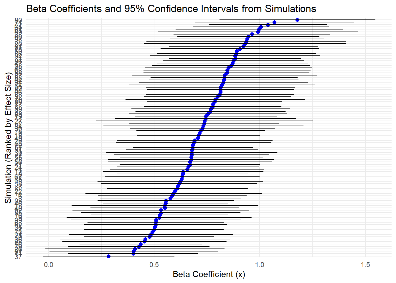

It looks like our simulation, on average, might be generating samples that overestimate the specified effect size. Perhaps we are generating too much random variation that, when applied to non-uniform baseline probabilities that cluster towards higher values, result in distributions that pull our beta estimates upwards? I am not entirely sure here, but let’s continue on.

13.4.3 collapsing & presenting dichotomous results

Recall, ultimately we want to compare probability of “agree” (y=4,5) versus “not agree” (1-3) categories across neighborhoods. To do that, we will need to collapse these outcome categories.

# Create a binary indicator for high agreement (4 or 5)
simdat <- simdat %>%
  mutate(high_agreement = ifelse(y %in% c(4, 5), 1, 0))

# Aggregate the proportion of high agreement responses by x
high_agreement_summary <- simdat %>%
  group_by(x) %>%
  summarise(
    high_agreement_proportion = mean(high_agreement),
    .groups = 'drop'
  )

# Check the aggregated data
high_agreement_summary

# A tibble: 2 × 2
  x     high_agreement_proportion
  <fct>                     <dbl>
1 0                         0.505
2 1                         0.63 

It seems the probability of agreement (y=4,5) is 12.5 percentage points higher in the x=1 neighborhoods than in the x=0 neighborhoods. Let’s plot this contrast.

# Plot the proportion of high agreement responses by neighborhood type
ggplot(high_agreement_summary, aes(x = as.factor(x), y = high_agreement_proportion, fill = as.factor(x))) +
  geom_bar(stat = "identity", width = 0.7, fill=c("maroon", "darkgrey")) +
  labs(
    title = "Proportion Agree Responses by Nbhd Risk",
    x = "Neighborhood Risk",
    y = "Proportion Agree Responses",
    fill = "Neighborhood Type"
  ) +
  scale_x_discrete(labels = c("0" = "At Risk", "1" = "Not at Risk")) +
  theme_minimal()

So, though the OR=1.5 and distributions varied, in this example the difference in probability of reporting “satisfied” categories is about 0.125 across neighborhood risk groups.

Recall, this is the type of contrast that we are likely to want to include for various item responses in our final report. We will return to this type of presentation later. First, let’s see if we can adjust our analysis to generate a power curve that displayes estimated power across different plausible effect magnitudes (odds ratios).

13.4.4 est. power across different plausible effect sizes

library(future)
library(furrr)

# Set up future for parallel processing
plan(multisession)  # or multicore depending on system

# Set simulation parameters
n_sim <- 100  # Number of simulations
alpha <- 0.05  # Significance level for hypothesis test
effect_sizes <- log(c(1.2, 1.3, 1.4, 1.5, 2))  # Different effect sizes to test (log-odds)

# Set other parameters for each simulation
n_neigh <- 40  # Number of neighborhoods
n_ind <- 20    # Number of individuals per neighborhood
n <- n_neigh * n_ind  # Total number of individuals
sigma_neigh <- 0.25  # Neighborhood random effect standard deviation
sigma_ind <- 1  # Individual-level noise

# Define the simulation function
run_simulation <- function(beta1) {
  tryCatch({
    # Simulate binary predictor ensuring equal split
    x_neigh <- rep(c(0, 1), each = n_neigh / 2)  # 20 "at risk" and 20 "not at risk"
    
    # Simulate neighborhood IDs
    neigh_id <- rep(1:n_neigh, each = n_ind)
    
    # Assign neighborhood-level x to individuals
    x <- rep(x_neigh, each = n_ind)
    
    # Generate neighborhood-level random intercepts
    neigh_intercept <- rnorm(n_neigh, mean = 0, sd = sigma_neigh)
    
    # Individual-level noise
    ind_noise <- rnorm(n, mean = 0, sd = sigma_ind)
    
    # Linear predictor (latent continuous variable)
    linpred <- beta1 * x + neigh_intercept[neigh_id] + ind_noise
    
    # Cut points (thresholds) for the ordinal outcome (logit-scale)
    cutpoints <- c(-1.5, -0.5, 0, 1.5)
    
    # Use the cut() function to assign categories
    y <- cut(linpred, breaks = c(-Inf, cutpoints, Inf), labels = 1:5, ordered_result = TRUE)
    
    # Combine into a data frame
    simdat <- data.frame(
      neigh_id = neigh_id,
      x = factor(x),  # Binary neighborhood predictor as factor
      y = factor(y, ordered = TRUE)  # Ordinal response variable
    )
    
    # Fit the cumulative link mixed model (CLMM) with neighborhood random effects
    fit <- clmm(y ~ x + (1 | neigh_id), data = simdat, control = clmm.control(maxIter = 100))
    
    # Extract the p-value for the predictor 'x'
    p_value <- summary(fit)$coefficients["x1", "Pr(>|z|)"]
    
    return(p_value)
  }, error = function(e) {
    # Return NA if any error occurs (model didn't fit)
    return(NA)
  })
}

# Function to estimate power for a given effect size
estimate_power <- function(beta1) {
  p_values <- future_map(1:n_sim, ~ run_simulation(beta1), .options = furrr_options(seed = TRUE))
  
  # Filter out NA values and count significant results
  valid_p_values <- p_values[!is.na(p_values)]
  significant_count <- sum(valid_p_values < alpha)
  
  # Calculate power as the proportion of significant results
  power <- significant_count / length(valid_p_values)
  
  return(power)
}

# Estimate power for different effect sizes
power_results <- future_map_dbl(effect_sizes, estimate_power, .options = furrr_options(seed = TRUE))

# Combine effect sizes and power results into a data frame
power_df <- data.frame(
  effect_size = effect_sizes,
  power = power_results
)

# Plot power by effect size
ggplot(power_df, aes(x = exp(effect_size), y = power)) +
  geom_line(color = "maroon", linewidth = 1) +
  geom_point(color = "black", size = 2) +
  labs(
    x = "Effect Size (Odds Ratio)",
    y = "Power",
    title = "Statistical Power by Effect Size"
  ) +
  theme_minimal()

If our simulation and modeling assumptions are reasonable then, based on this plot, our research design affords an estimated >=80% power to detect effects approximately OR=1.35 or larger at an alpha level of 0.05.

13.4.5 visualizing minimum detectable effect at est. 80% power (OR=1.35)

One more thing. How large might an odds ratio of 1.35 be in a predicted probability metric? We can estimate and plot such hypothetical differences using the baseline response probability thresholds specified in the simulation. Let’s do this with a full ordinal distribution and after collapsing categories into dichotomous agree/not agree response distributions. This will help us visualize the magnitude of hypothetical contrasts that we might have sufficient power to detect in this study.

library(patchwork)

# Thresholds (cutpoints) from the simulation
thresholds <- c(-1.5, -0.5, 0, 1.5)

# Effect size (log odds for x=1)
log_odds_ratio <- log(1.35)

# Linear predictor for x=0 (at risk) and x=1 (not at risk)
eta_0 <- 0
eta_1 <- log_odds_ratio

# Logistic function to calculate cumulative probabilities
logistic <- function(x) {
  return(1 / (1 + exp(-x)))
}

# Calculate cumulative probabilities for each group
cum_probs_0 <- logistic(thresholds - eta_0)
cum_probs_1 <- logistic(thresholds - eta_1)

# Calculate predicted probabilities (P(y = k))
probs_0 <- c(cum_probs_0[1], diff(cum_probs_0), 1 - cum_probs_0[4])
probs_1 <- c(cum_probs_1[1], diff(cum_probs_1), 1 - cum_probs_1[4])

# Collapse the categories y = 1,2,3 and y = 4,5
collapsed_probs_0 <- c(sum(probs_0[1:3]), sum(probs_0[4:5]))
collapsed_probs_1 <- c(sum(probs_1[1:3]), sum(probs_1[4:5]))

# Create a data frame for full ordinal plot
pred_prob_df <- data.frame(
  category = factor(1:5),
  prob_x0 = probs_0,  # At risk (x=0)
  prob_x1 = probs_1   # Not at risk (x=1)
) %>%
  pivot_longer(cols = starts_with("prob"), names_to = "group", values_to = "probability") %>%
  mutate(group = recode(group, "prob_x0" = "At Risk (x=0)", "prob_x1" = "Not at Risk (x=1)"))

# Create a data frame for the collapsed categories
collapsed_prob_df <- data.frame(
  category = factor(c("y=1,2,3", "y=4,5")),
  prob_x0 = collapsed_probs_0,  # At risk (x=0)
  prob_x1 = collapsed_probs_1   # Not at risk (x=1)
) %>%
  pivot_longer(cols = starts_with("prob"), names_to = "group", values_to = "probability") %>%
  mutate(group = recode(group, "prob_x0" = "At Risk (x=0)", "prob_x1" = "Not at Risk (x=1)"))

# Plot full predicted probabilities for x=0 and x=1
plot1 <- ggplot(pred_prob_df, aes(x = category, y = probability, fill = group)) +
  geom_bar(stat = "identity", position = "dodge", width = 0.7) +
  scale_fill_manual(values = c("maroon", "darkgrey")) +
  labs(
    x = "Ordinal Outcome (y)",
    y = "Predicted Probability"
  ) +
  theme_minimal()

# Plot collapsed predicted probabilities for x=0 and x=1
plot2 <- ggplot(collapsed_prob_df, aes(x = category, y = probability, fill = group)) +
  geom_bar(stat = "identity", position = "dodge", width = 0.7) +
  scale_fill_manual(values = c("maroon", "darkgrey")) +
  labs(
    x = "Collapsed Ordinal Outcome",
    y = "Predicted Probability"
  ) +
  theme_minimal()

plot1 + plot2 + 
  plot_layout(guides = "collect") +
   plot_annotation(
     title = "Simulated Pred. Prob. Contrasts by Nbhd Risk Group", 
     subtitle = "Est. 80% power to detect this hypothetical contrast of OR=1.35") &
  theme(legend.position = "bottom")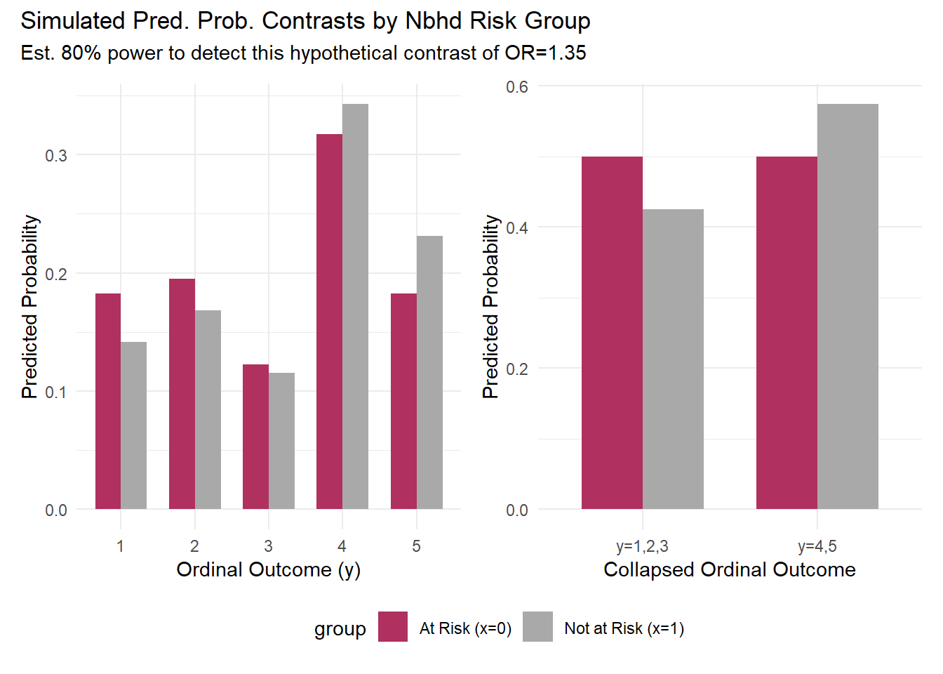 

13.4.6 summary table

# Create summary table of power results
power_summary <- data.frame(
  Odds_Ratio = exp(effect_sizes),
  Log_Odds = effect_sizes,
  Power = power_results
) %>%
  mutate(
    Adequate_Power = ifelse(Power >= 0.8, "Yes", "No"),
    Power_Percent = paste0(round(Power * 100, 1), "%")
  )

knitr::kable(power_summary, 
             caption = "Statistical Power by Effect Size (OR)",
             digits = 3)

Statistical Power by Effect Size (OR)

Odds_Ratio	Log_Odds	Power	Adequate_Power	Power_Percent
1.2	0.182	0.43	No	43%
1.3	0.262	0.68	No	68%
1.4	0.336	0.88	Yes	88%
1.5	0.405	0.96	Yes	96%
2.0	0.693	1.00	Yes	100%

Based on these simulations, the proposed design (n=800, 40 neighborhoods, 20 participants per neighborhood) provides adequate power (≥80%) to detect effect sizes of OR=1.35 or larger. In practical terms, this corresponds to detecting differences of approximately 6-9 percentage points in ‘agreement’ rates between high-crime and random sample neighborhoods.

Brauer, Jonathan, and Jacob Day. 2025. “Pursuing Precision in Criminology: Why Ordinal Data Demand Ordinal Methods.” OSF. https://doi.org/10.31235/osf.io/fet4d_v1.

Day, Jake, Jon Brauer, and Maja Kotlaja. 2023. “Trust Issues: Examining Near Duplicates in Survey Data.” https://reluctantcriminologists.com/blog-posts/%5B8%5D/dup-series/duplicates.

Kuriakose, Noble, and Michael Robbins. 2015. “Don’t Get Duped: Fraud Through Duplication in Public Opinion Surveys.” {SSRN} {Scholarly} {Paper}. Rochester, NY: Social Science Research Network. https://papers.ssrn.com/abstract=2580502.

Revelle, William. 2024. “The Seductive Beauty of Latent Variable Models: Or Why I Don’t Believe in the Easter Bunny.” Personality and Individual Differences 221 (April): 112552. https://doi.org/10.1016/j.paid.2024.112552.

Sampson, Robert J., Stephen W. Raudenbush, and Felton Earls. 1997. “Neighborhoods and Violent Crime: A Multilevel Study of Collective Efficacy.” Science 277 (5328): 918–24. https://doi.org/10.1126/science.277.5328.918.

Wheeler, Andrew. 2023. “Survey Duplicates and Other Stuff.” Andrew Wheeler. https://andrewpwheeler.com/2023/10/13/survey-duplicates-and-other-stuff/.

---

1. For the sake of transparency, we do not think statistical power estimates or statistical inferences based on null hypothesis significance testing are usually very useful in typical quantitative applications in our field. To be sure, they are quite important in fields and applications where researchers are testing a small number of very precisely articulated (point, range, or equivalence) hypotheses, usually with experimental or quasi-experimental designs, and where prior tests exist that can provide precise information to inform assumptions about things like expected baseline probabilities, individual- and group-level variation, and smallest effect size of interest in context, in addition to (especially in observational designs) well-articulated causal theoretical expectations about potential confounds, mediators, effect heterogeneity and moderators, and so on. In contexts lacking precise hypotheses to test and precise prior information to inform tests and designs, we are skeptical that the numeric quantities generated by an a priori power analysis are likely to precisely match the true power of any subsequent “test” - particularly because such research at best is likely to generate theoretically-informed descriptive inferences rather than strict hypothesis tests. With that said, we realize that researchers often are encouraged or required to conduct a priori power analysis, and we certainly see value in thinking through one’s design, anticipated data, intended modeling approach, desired estimand, and related assumptions following from these decisions and practices. So, despite our typical reservations, we gave it the old college try.