RRR: Mediation Makes My Head Hurt!

Our first Reluctantly Rapid Response (RRR) post addresses a confusing mediation issue.

Mediation makes my head hurt

Motivation

At times, we find ourselves wanting to publish a brief or “quick hitting” entry with a brief comment or coding example but do not have the time for a formal blog post. So, we decided to pilot a new type of entry. For lack of a better term, we’ll call this a “Reluctantly Rapid Response” (RRR for short). We are generally reluctant to post anything and doubly reluctant to post anything rapidly, so the name seems fitting to us.

This RRR entry provides code and output from a simple simulation motivated by Brier Gallihugh’s question on X about a mediation issue.

A mediation mystery unfolds

The following simulation, plots, and analysis provide one example situation in which changes in a mediator (ChgM) are positively correlated with changes in an outcome (ChgY) within two groups A & B, yet Group A membership is estimated as having a negative indirect effect on changes in the outcome (ChgY) via changes in the mediator (ChgM). In this example, the total negative indirect effect is generated by a small negative “pure” indirect (PNIE) effect combined with a small “mediated interaction” (INTmed) effect.

I am not claiming that this is what is happening in the original poster’s (BG’s) data. In fact, one apparent and important difference is that BG stated in a later tweet that “Group A shows higher rates of their mediator compared to Group B AND lower rates of the outcome compared to Group B as well.”

The probability plot thickens

If “rates” refer to initial status at Time 1 (not changes), then perhaps we could generate comparable data. Yet, if “rates” refers to the change scores themselves, then it seems we may still have an unsolved problem on our hands. In the simulation below, changes in the mediator are positively correlated with changes in the outcome in both Groups A and B, and Group A has lower outcome change scores on average; however, specification of marginally lower mediator change scores on average for Group A contribute to the negative indirect effect estimates.

Please feel free to reach out on X or via email if you see errors or have other suggestions!

Load libraries

library(tidyverse)
library(ggplot2)
library(patchwork)
library(psych)
# library(devtools)
# install_github("jtextor/dagitty/r")
library(dagitty)
library(CMAverse)

Basic DAG

SimpsonDAG <- dagitty("dag{
  GroupA -> ChgM -> ChgY
  GroupA -> ChgY
   }") 
coordinates(SimpsonDAG) <- list(
  x=c(GroupA=1, ChgM=2, ChgY=3),
  y=c(GroupA=2, ChgM=1, ChgY=2) )

plot(SimpsonDAG)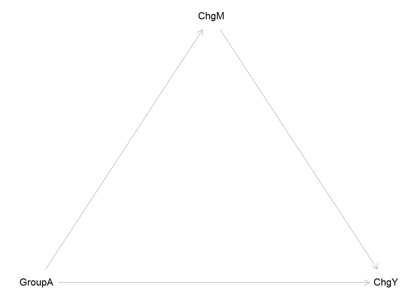

Simulate data

set.seed(1138)
n <- 500
GroupA<-rbinom(n=1000,size=1,prob=0.50)
ChgM <- -.1*GroupA + rnorm(n)
ChgY <- .5*ChgM + -.5*GroupA + .4*GroupA*ChgM + rnorm(n)
simdata <- tibble(GroupA, ChgM, ChgY)

simdata

# A tibble: 1,000 × 3
   GroupA   ChgM    ChgY
    <int>  <dbl>   <dbl>
 1      0 -0.358  0.687 
 2      0 -0.490 -2.07  
 3      0 -0.115  0.895 
 4      1 -0.451 -1.65  
 5      1 -0.588 -1.31  
 6      0 -0.961  0.371 
 7      1 -0.732 -1.51  
 8      1  0.294 -0.344 
 9      0 -0.249  0.0797
10      1 -2.42  -2.25  
# ℹ 990 more rows

GroupAplot <- simdata %>% ggplot() +
  geom_bar(aes(x=GroupA),
                 color="#1fa187", fill="#4ac16d", alpha=.7,
                 position="identity") + 
  theme_minimal() + 
  theme(axis.text.y=element_blank(),  
        axis.ticks.y=element_blank()
        ) +
  labs(x="GroupA", y=NULL)

ChgMplot <- simdata %>% ggplot() +
  geom_histogram(aes(x=ChgM, y=..density..),
                 color="#1fa187", fill="#4ac16d", alpha=.7,
                 position="identity", 
                 breaks = seq(-4, 4, by = 1)) + 
  theme_minimal() + 
  theme(axis.text.y=element_blank(),  
        axis.ticks.y=element_blank()
        ) +
  labs(x="ChgM", y=NULL)

ChgYplot <- simdata %>% ggplot() +
  geom_histogram(aes(x=ChgY, y=..density..),
                 color="#1fa187", fill="#4ac16d", alpha=.7,
                 position="identity") + 
  theme_minimal() + 
  theme(axis.text.y=element_blank(),  
        axis.ticks.y=element_blank()
        ) +
  labs(x="ChgY", y=NULL)


GroupAplot + ChgMplot + ChgYplot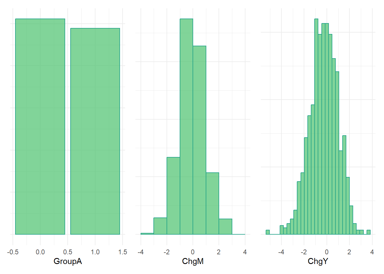

Bivariate corrs

Full sample

Positive correlation between ChgM and ChgY in full sample.

pairs.panels(simdata,
             smooth = FALSE,      # If TRUE, draws loess smooths
             scale = FALSE,      # If TRUE, scales the correlation text font
             density = TRUE,     # If TRUE, adds density plots and histograms
             ellipses = FALSE,    # If TRUE, draws ellipses
             method = "pearson", # Correlation method (also "spearman" or "kendall")
             pch = 21,           # pch symbol
             lm = TRUE,         # If TRUE, plots linear fit rather than the LOESS (smoothed) fit
             cor = TRUE,         # If TRUE, reports correlations
             jiggle = FALSE,     # If TRUE, data points are jittered
             factor = 2,         # Jittering factor
             hist.col = 3,       # Histograms color
             stars = TRUE,       # If TRUE, adds significance level with stars
             ci = TRUE)          # If TRUE, adds confidence intervals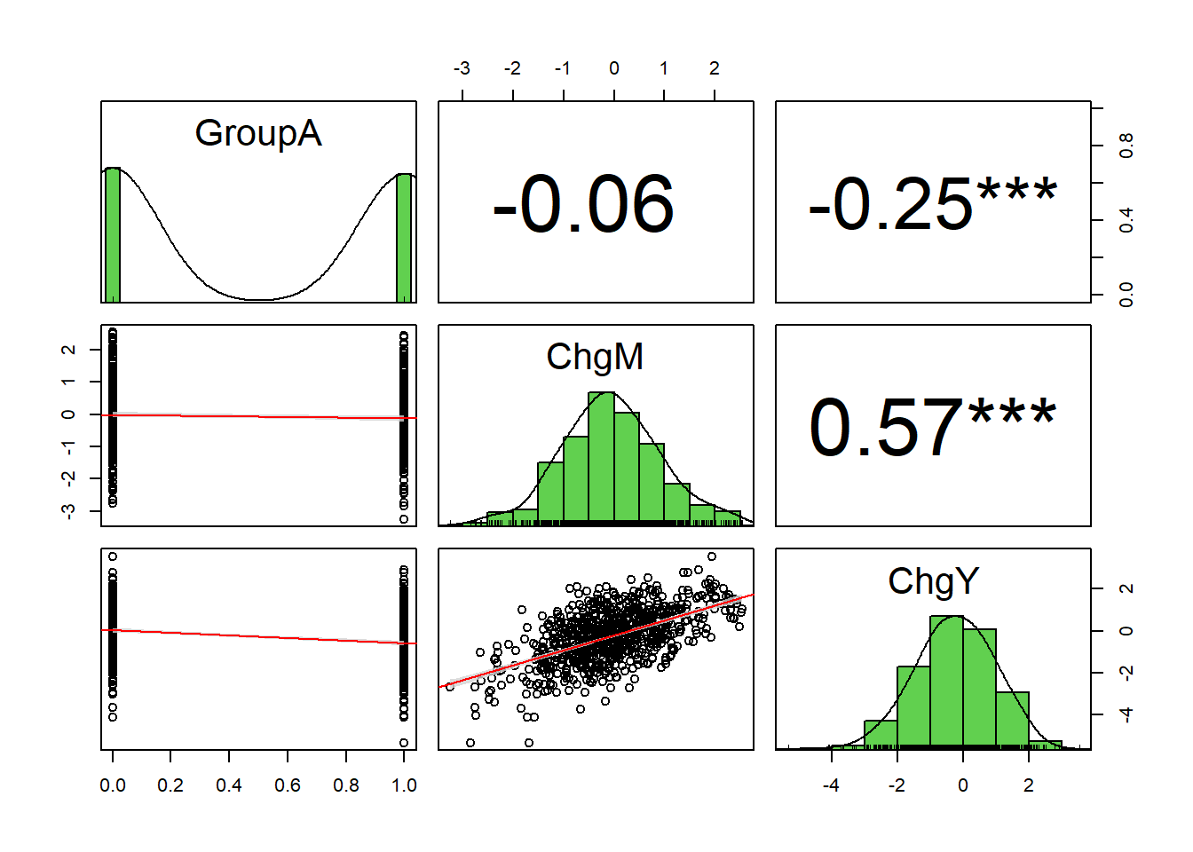

Group A only

Positive correlation between ChgM and ChgY within Group A.

simdataA <- simdata %>% filter(GroupA==1) %>% select(-GroupA)
pairs.panels(simdataA, density = TRUE, method = "pearson", pch = 21, 
             lm = TRUE, cor = TRUE, hist.col = 3, stars = TRUE, ci = TRUE)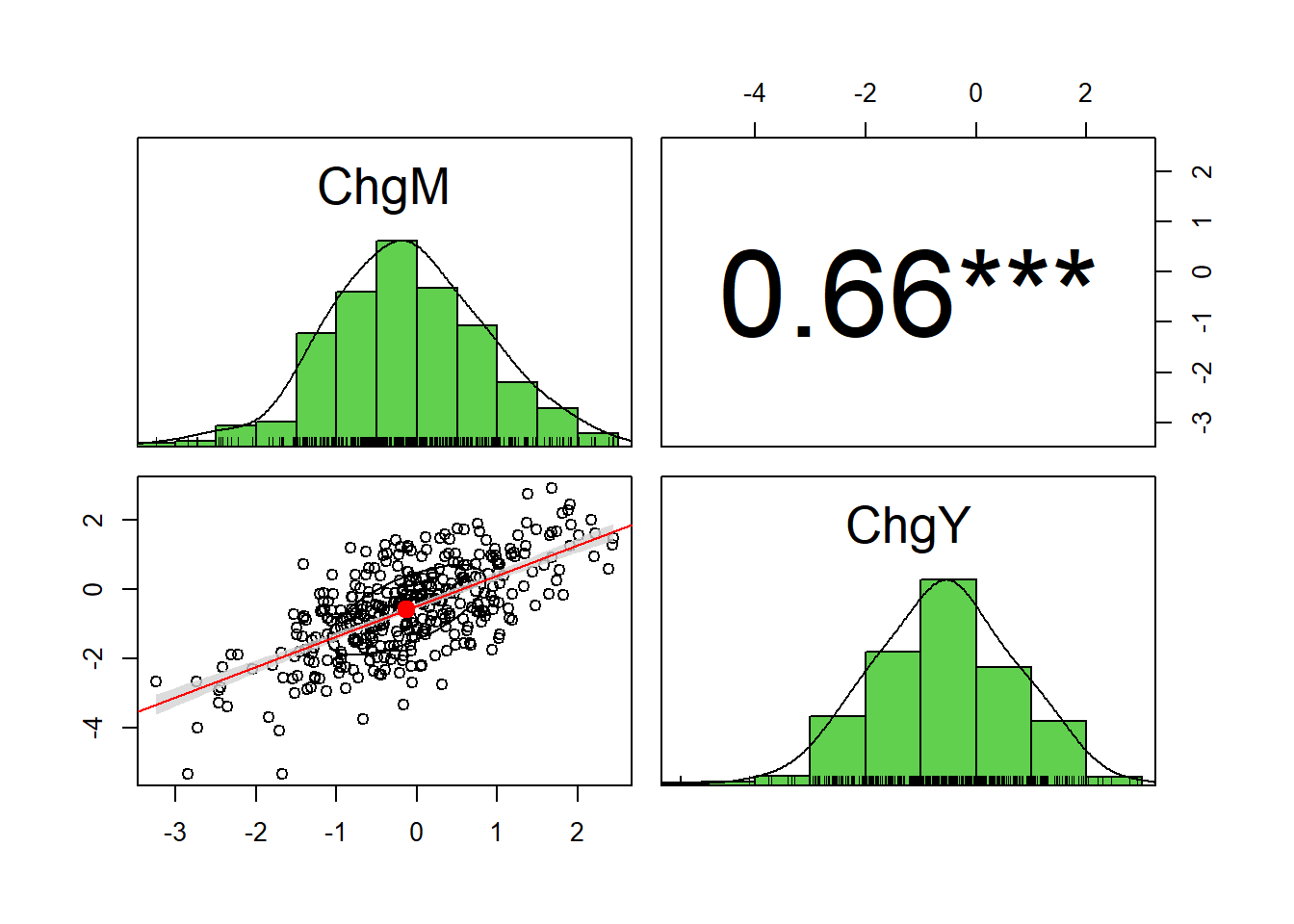  

Group B only

Positive correlation between ChgM and ChgY within Group B.

simdataB <- simdata %>% filter(GroupA==0) %>% select(-GroupA)
pairs.panels(simdataB, density = TRUE, method = "pearson", pch = 21, 
             lm = TRUE, cor = TRUE, hist.col = 3, stars = TRUE, ci = TRUE)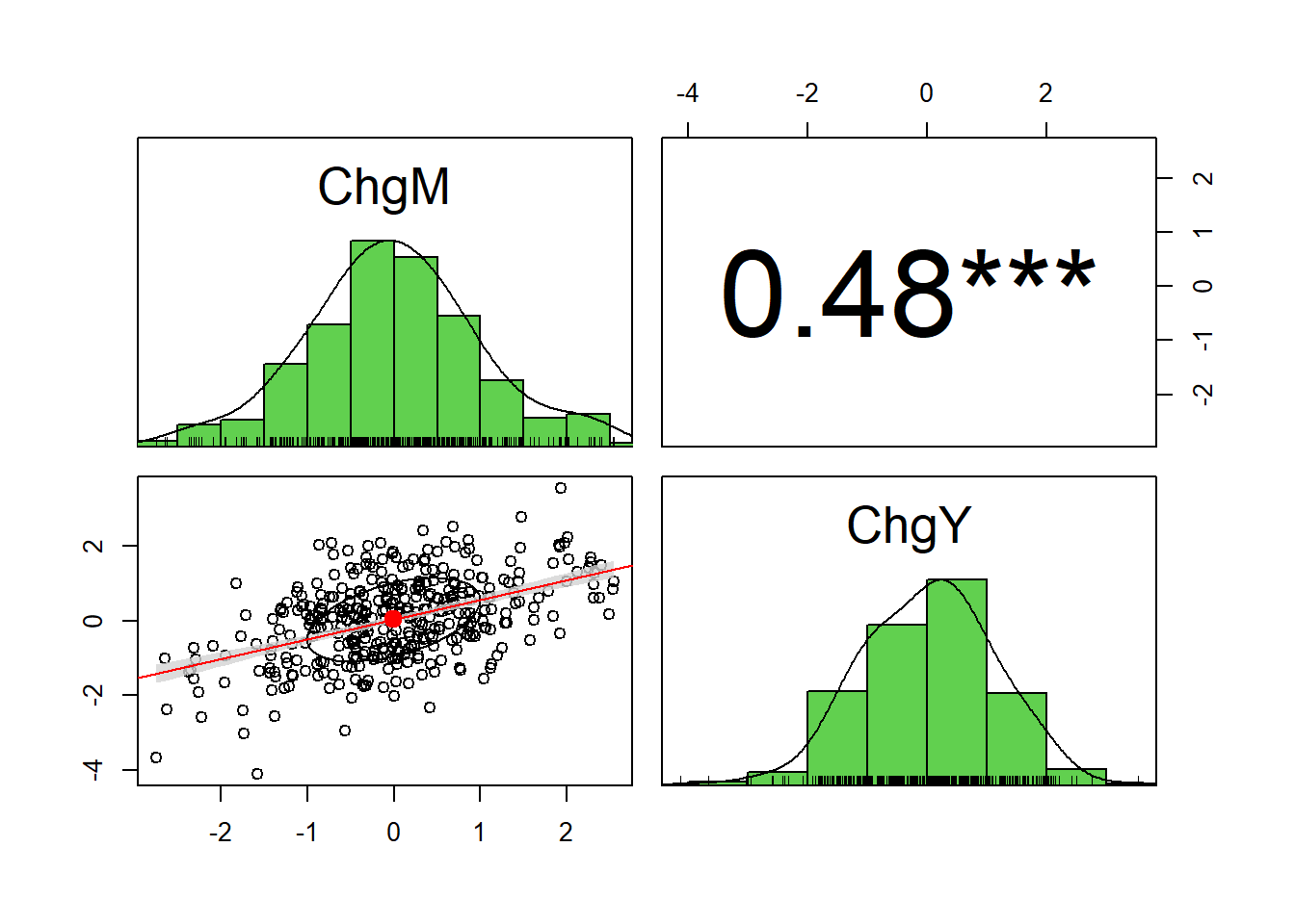  

Scatterplot by group

Notice inconsistent or heterogeneous effect of ChgM on ChgY across Groups.

ggplot(data = simdata, aes(x = ChgM, y = ChgY)) +
        geom_point(aes(shape = factor(GroupA))) +
        geom_point(aes(color = factor(GroupA))) +
        geom_smooth(method = "lm", 
                    se = FALSE, 
                    aes(color = factor(GroupA)))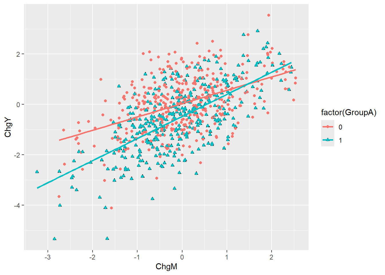 

Simple mediation model

Negative indirect effect of GroupA on ChgY via ChgM.

mediate(ChgY ~ GroupA + (ChgM), data = simdata, n.iter = 10000) %>% print(short = TRUE)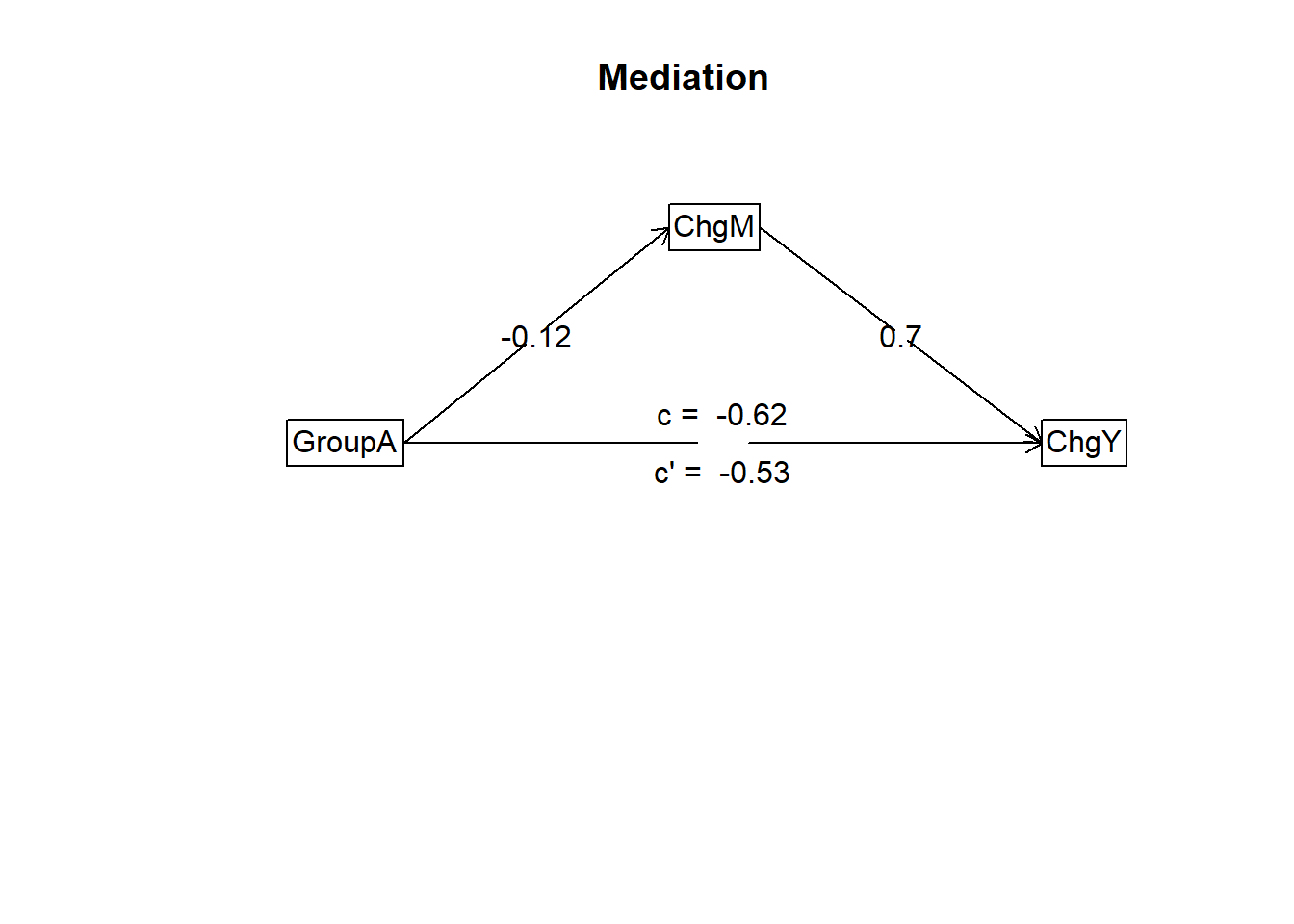

Mediation/Moderation Analysis 
Call: mediate(y = ChgY ~ GroupA + (ChgM), data = simdata, n.iter = 10000)

The DV (Y) was  ChgY . The IV (X) was  GroupA . The mediating variable(s) =  ChgM .

Total effect(c) of  GroupA  on  ChgY  =  -0.62   S.E. =  0.08  t  =  -8.07  df=  998   with p =  2e-15
Direct effect (c') of  GroupA  on  ChgY  removing  ChgM  =  -0.53   S.E. =  0.06  t  =  -8.47  df=  997   with p =  8.5e-17
Indirect effect (ab) of  GroupA  on  ChgY  through  ChgM   =  -0.08 
Mean bootstrapped indirect effect =  -0.08  with standard error =  0.04  Lower CI =  -0.17    Upper CI =  0
R = 0.61 R2 = 0.37   F = 289.17 on 2 and 997 DF   p-value:  5.13e-135 

 To see the longer output, specify short = FALSE in the print statement or ask for the summary

Mediation model accounting for exposure-mediator interaction

Total negative indirect effect (PNIE + INTmed) estimate is larger after accounting for exposure-mediator interaction.

set.seed(1138)
est <- cmest(data = simdata, model = "rb", outcome = "ChgY", exposure = "GroupA",
                mediator = "ChgM", EMint = TRUE,
                mreg = list("linear"), yreg = "linear",
                astar = 0, a = 1, mval = list(0),
                estimation = "imputation", inference = "bootstrap", nboot = 20)

  |                                                                            
  |                                                                      |   0%
  |                                                                            
  |====                                                                  |   5%
  |                                                                            
  |=======                                                               |  10%
  |                                                                            
  |==========                                                            |  15%
  |                                                                            
  |==============                                                        |  20%
  |                                                                            
  |==================                                                    |  25%
  |                                                                            
  |=====================                                                 |  30%
  |                                                                            
  |========================                                              |  35%
  |                                                                            
  |============================                                          |  40%
  |                                                                            
  |================================                                      |  45%
  |                                                                            
  |===================================                                   |  50%
  |                                                                            
  |======================================                                |  55%
  |                                                                            
  |==========================================                            |  60%
  |                                                                            
  |==============================================                        |  65%
  |                                                                            
  |=================================================                     |  70%
  |                                                                            
  |====================================================                  |  75%
  |                                                                            
  |========================================================              |  80%
  |                                                                            
  |============================================================          |  85%
  |                                                                            
  |===============================================================       |  90%
  |                                                                            
  |==================================================================    |  95%
  |                                                                            
  |======================================================================| 100%

summary(est)

Causal Mediation Analysis

# Outcome regression:

Call:
glm(formula = ChgY ~ GroupA + ChgM + GroupA * ChgM, family = gaussian(), 
    data = getCall(x$reg.output$yreg)$data, weights = getCall(x$reg.output$yreg)$weights)

Coefficients:
            Estimate Std. Error t value Pr(>|t|)    
(Intercept)  0.03308    0.04337   0.763    0.446    
GroupA      -0.51010    0.06229  -8.190 7.97e-16 ***
ChgM         0.53021    0.04329  12.248  < 2e-16 ***
GroupA:ChgM  0.34764    0.06259   5.554 3.58e-08 ***
---
Signif. codes:  0 '***' 0.001 '**' 0.01 '*' 0.05 '.' 0.1 ' ' 1

(Dispersion parameter for gaussian family taken to be 0.9610836)

    Null deviance: 1559.35  on 999  degrees of freedom
Residual deviance:  957.24  on 996  degrees of freedom
AIC: 2804.2

Number of Fisher Scoring iterations: 2


# Mediator regressions: 

Call:
glm(formula = ChgM ~ GroupA, family = gaussian(), data = getCall(x$reg.output$mreg[[1L]])$data, 
    weights = getCall(x$reg.output$mreg[[1L]])$weights)

Coefficients:
             Estimate Std. Error t value Pr(>|t|)  
(Intercept) -0.006556   0.043905  -0.149   0.8813  
GroupA      -0.120841   0.062786  -1.925   0.0546 .
---
Signif. codes:  0 '***' 0.001 '**' 0.01 '*' 0.05 '.' 0.1 ' ' 1

(Dispersion parameter for gaussian family taken to be 0.9850333)

    Null deviance: 986.71  on 999  degrees of freedom
Residual deviance: 983.06  on 998  degrees of freedom
AIC: 2826.8

Number of Fisher Scoring iterations: 2


# Effect decomposition on the mean difference scale via the regression-based approach
 
Direct counterfactual imputation estimation with 
 bootstrap standard errors, percentile confidence intervals and p-values 
 
              Estimate Std.error   95% CIL 95% CIU  P.val    
cde          -0.510101  0.073753 -0.651063  -0.410 <2e-16 ***
pnde         -0.514441  0.074196 -0.638106  -0.410 <2e-16 ***
tnde         -0.556449  0.076406 -0.692366  -0.431 <2e-16 ***
pnie         -0.064071  0.034397 -0.126845  -0.011 <2e-16 ***
tnie         -0.106080  0.056820 -0.194148  -0.019 <2e-16 ***
te           -0.620520  0.089392 -0.778236  -0.465 <2e-16 ***
intref       -0.004339  0.015854 -0.029367   0.025    0.8    
intmed       -0.042009  0.025189 -0.095535  -0.008 <2e-16 ***
cde(prop)     0.822054  0.068527  0.730253   0.935 <2e-16 ***
intref(prop)  0.006993  0.025298 -0.042487   0.047    0.8    
intmed(prop)  0.067700  0.035646  0.017009   0.143 <2e-16 ***
pnie(prop)    0.103254  0.047652  0.021586   0.183 <2e-16 ***
pm            0.170953  0.078667  0.038596   0.283 <2e-16 ***
int           0.074693  0.031196  0.022878   0.120 <2e-16 ***
pe            0.177946  0.068527  0.064943   0.270 <2e-16 ***
---
Signif. codes:  0 '***' 0.001 '**' 0.01 '*' 0.05 '.' 0.1 ' ' 1

(cde: controlled direct effect; pnde: pure natural direct effect; tnde: total natural direct effect; pnie: pure natural indirect effect; tnie: total natural indirect effect; te: total effect; intref: reference interaction; intmed: mediated interaction; cde(prop): proportion cde; intref(prop): proportion intref; intmed(prop): proportion intmed; pnie(prop): proportion pnie; pm: overall proportion mediated; int: overall proportion attributable to interaction; pe: overall proportion eliminated)

Relevant variable values: 
$a
[1] 1

$astar
[1] 0

$mval
$mval[[1]]
[1] 0